How many conserved quantities are there?

In classical Newtonian mechanics as taught in high school, we're familiar with various conserved quantities: The most important ones are energy, momentum and angular momentum. In a more sophisticated setting, we think of these as due to certain symmetries of the system or its Lagrangian. Energy conservation is due to time translation symmetry, momentum conservation is due to spatial translation symmetry, and angular momentum conservation is due to rotational symmetry.

A couple of years ago (2021), I noticed a pattern about the character of these conserved quantities in the context of geometric algebra (or more generally Clifford algebra):

Let's look at a particle freely moving in 1D space. The system has two conserved quantities:

1. The energy of the particle, which is a scalar quantity.

$E = \frac{p^2}{2m} + V(x)$

2. The momentum of the particle, which is a vector quantity.

$p = m v$

Now let's look at a particle freely moving in 2D space. The system has three conserved quantities, one more than in 1D:

1. The energy of the particle, which is a scalar quantity.
2. The momentum of the particle.
3. The angular momentum of the particle, which is a bivector (or pseudovector) quantity. $\mathbf{L} = \mathbf{r} \wedge \mathbf{p}$

We often think of the angular momentum as a vector $\vec{x} \times \vec{p}$ in 3D, but in fact it stems from a bivector $\vec{x} \wedge \vec{p}$, which is a 2D conserved area. The two are related through a Hodge dual, $\star(\vec{x} \wedge \vec{p}) = \vec{x} \times \vec{p}$, which maps areas onto surfaces. This works because there are three orthogonal vectors and three orthogonal planes in 3D, so each bivector can be mapped onto the vector in the orthogonal direction. Kepler's second law that a constant area swept out by an orbit over time makes this very apparent and is a very natural consequence of the conserved angular momentum being an area-like bivector quantity.

This pattern seems to hold in a more complicated case, e.g. that of two orbiting bodies. The system can be reduced to two dimensions, parametrized e.g. by the distance and angle between the bodies. Just like for the free 2D particle, we get tgree conserved quantities:

1. The total energy, a scalar quantity.

$E = \frac{p^2}{2m} + V(\mathbf{r})$

2. The Laplace-Runge-Lenz vector.

$\mathbf{A} = \mathbf{p} \times \mathbf{L} - m k \frac{\mathbf{r}}{|\mathbf{r}|}$

Despite the cross product, this object is in fact a vector, not a bivector, and can be expressed in terms of the following wedge product:

$\mathbf{A} = \star \left[ \mathbf{p} \wedge \star(\mathbf{r} \wedge \mathbf{p}) \right] - m k \frac{\mathbf{r}}{|\mathbf{r}|}$

3. The system's angular momentum.

For completeness, a particle in 0D can be seen as having only a single (somewhat trivial as there's no space to move through!) conserved quantity, a scalar energy, but no momentum vector or angular momentum bivector because there's no vector space for these quantities to exist in.

For each additional dimension we seem to get a new conserved quantity! Can we extend this to 3D?

In the 3D case there are no fundamental physical conserved quantities that immediately come to mind, but for example: We can also think of the trivector $\vec{x} \wedge \vec{y} \wedge \vec{z}$, which defines the orientation or handedness of the coordinate axes relative to each other. This trivector can be converted into a pseudoscalar through a Hodge dual, and in that form can take the value +1 or -1 depending on the orientation of the coordinate system. So this is another conserved quantity which is volume-like. More examples later.

The overall pattern seems that in higher dimensions, we get one conserved quantity for each additional grade of blades in the algebra. This would mean that in $n$D, we'd have:

• Scalar energy
• Vector momentum
• Bivector angular momentum
• Trivector (or 3D) conserved volume of some sort
• Quad-vector (or 4D) conserved hypervolume of some sort
• ...
• $n-1$ D conserved $n-1$ D volume (or pseudovector) of some sort
• $n$ D conserved $n$ D volume (or pseudoscalar) of some sort

What's also apparent from the Keplerian example is that the conserved quantities can take an unexpected form like the Laplace-Runge-Lenz vector. This indicates that there may still be conserved quantities in systems that don't have a clear symmetry, so maybe each system has a fixed number of them but they are non-trivial to express or find, but an existance proof could be given by the dimensionality of the system.

This hypothesis is cool because it would predict that there are more conserved quantities in higher dimensions, and we might be able to understand them in terms of the allowed grades, or as part of a single conserved multivector unifying all of them into one object.

While it turns out that this hypothesis is wrong in this formulation, but it's wrong in interesting ways that are worth talking about. In particular, going through this exercise helped me more clearly understand the nuances of constants of integration, conserved quantities (Noether charges), gauges and scale invariance (internal and external), and what the Buckingham $\Pi$ theorem really tells us. This should be quite the ride.

Support for higher grade conserved quantities

Digging through the literature, I found it hard to find examples of higher grade conserved quantities in classical mechanics, and no clear writeup of the pattern or a clear conterfactual. I did find something in a book Geometric Algebra for Physicists, Chapter 9 in a section on invariants a relativistic two-particle (maximally entangled) singlet state. A table summarizes the relativistic invariants of the system, which follow the pattern of one invariant for each grade of the algebra.

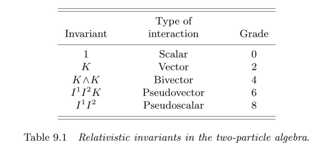
The invariants here are constructed from the basis vectors $\gamma_{\mu}^1$ and $\gamma_{\nu}^2$ of two copies of the spacetime vector basis sets, one for each particle. This purely geometric construction produces a series of quantities of increasing grade that are invariant under Lorentz boosts. They are, however, not necessarily conserved quantities in the sense of Noether's theorem, and they are not generators of any symmetries.

Also in the context of special relativity, there is the Pauli–Lubanski pseudovector, which is a legitimate conserved quantity. We can construct the Pauli–Lubanski pseudovector like this:

$W_{\mu} = \frac{1}{2}\,\varepsilon_{\mu\nu\rho\sigma}\,J^{\nu\rho}\,P^{\sigma} = \frac{1}{6} \varepsilon_{\mu\nu\rho\sigma}\,(J \wedge P)^{\nu\rho\sigma}$

where $P^{\mu}$ is the relativistic 4-momentum and $J^{\mu\nu}$ the angular momentum tensor as the sum of the orbital angular momentum and intrinsic spin:

$J^{\mu\nu} \;=\; (x \wedge P)^{\mu\nu} \;+\; S^{\mu\nu} \;=\; x^\mu P^\nu - x^\nu P^\mu + S^{\mu\nu}\,,$

or because $x \wedge P \wedge P = 0$:

$J\wedge P=\bigl(x\wedge P + S\bigr)\wedge P=x\wedge P\wedge P \;+\;S\wedge P=S\wedge P,$

so

$W=\star\bigl(J\wedge P\bigr)=\star\bigl(S\wedge P\bigr).$

The Pauli–Lubanski pseudovector is called pseudovector because it is actually the Hodge dual of a trivector. This construction commutes with the Hamiltonian (as $J$ and $P$ both commute) and is a conserved quantity. On its own it's not Lorentz invariant, but $W^2 = W_{\mu} W^{\mu}$ is. However, it's also one of the two Casimir invariants of the Poincaré group, alongside $P^2$. These two operators are part of the center of the algebra, which means they commute with all other operators, and thus behave like the identity times some scalar Because of this they only give rise to trivial symmetries, and the Pauli–Lubanski pseudovector is a conserved quantity, but not a symmetry generator.

As some non-relativistic examples, there are several pseodoscalar quantities in 3D systems that correspond to Hodge duals of trivectors:

One prominent example is the helicity of a fluid flow. Under the Euler equation in hydrodynamics an ideal, incompressible, inviscid fluid with velocity field $\mathbf{u}(\mathbf{x},t)$ and vorticity $\boldsymbol\omega = \nabla\times\mathbf{u}$, has a helicity density:

$H_{\!m} = \int d^3x\;\mathbf{A}\cdot\mathbf{B} = \frac12\int d^3x\;\varepsilon_{ijk}\,A_i\,B_{jk},$

or for the trivector:

$\mathcal{H}_{\rm fluid}=u\wedge du$

An analog of this is the magnetic helicity in electromagnetism, the integral over which is a conserved quantity in the absence of resistivity. The vector potential

$\mathcal{H}_{\rm mag}=A\wedge F = A \wedge dA = \frac{\partial A_{k}}{\partial x^{j}}\,A \wedge dx^{j}\wedge dx^{k} \;=\; ...$

$\;=\; A_i\,\partial_jA_k\;dx^i\wedge dx^j\wedge dx^k$

After integration both retain their pseudoscalar character, and are conserved quantities:

$x\rightarrow-x,\; y\rightarrow-y, \; z\rightarrow-z \quad\Longrightarrow\quad H\rightarrow-\,H,$

transforming like a volume (unlike energy which is invariant under parity).

One final example is the phase space volume of a system of $n$ particles in 3D, which is conserved under Liouville's theorem:

$\Omega = \underbrace{dq^1\wedge dp_1\wedge \cdots\wedge dq^n\wedge dp_n}_{\text{\(2n\)-form}}.$

More generally, incompressible, divergence-free flows (i.e. $\nabla\cdot\mathbf{v}=0$) preserve volumes by definition.

What exactly is a conserved quantity?

One thing I realized is that what exactly I'm mean when I say "conserved quantities" is not so clear. In different context, this can mean different things. I'll briefly mention here what I see as the main distinctions and notions of symmetry they're associated with. Then we'll go into detail on each type and how they relate to the question at hand in the next sections.

Conserved quantities:

• Noether charges: these are conserved quantities that arise from symmetries of the system, and are related to the invariance of the action under continuous transformations.
• Constants of integration: these are quantities that arise from the integration of differential equations.
• Invariants: these are quantities that are invariant under certain transformations, and can be related to the symmetries of the system.

Symmetries:

• Gauge symmetries: these are symmetries that arise from the invariance of the system under gauge transformations, and are related to the redundancy of the description of the system. There are internal gauge symmetries and external gauge symmetries.
• Scale symmetries: these are symmetries that arise from the invariance of the system under scaling transformations, and are related to the dimensionality of the system.
• Global symmetries: these are symmetries that arise from the invariance of the system under global transformations. These give rise to Noether charges.
• Local symmetries: these are symmetries that arise from the invariance of the system under local transformations, and are related to the local properties of the system.

Stone's theorem: Unitary transformations and exponential famlilies

In many quantum mechanics classes, Stone's theroem is introduced as a connection between unitary (Hermitian) operators and a family of exponentials: any strongly continuous family of unitaries $U(t)$ can be written

$U(t) \;=\; e^{-i\,t\,H},$

where $H$ is self-adjoint. The factor of $i$ ensures unitarity; equivalently, one can say the Hermitian operator $H$ generates the flow.

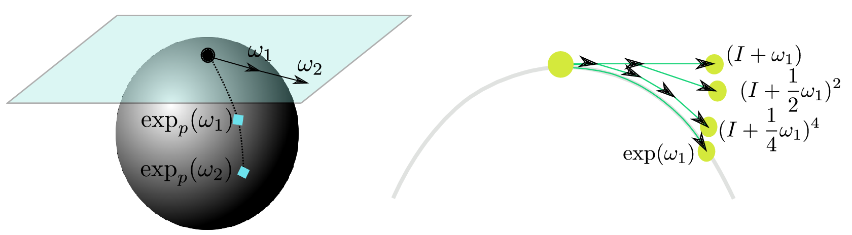
This statement be intuitively understood in a more general context as an application of the Euler method for differential equations: We start with a differential equation:

$\frac{dy}{dt} = f(y, t), \quad y(t_0) = y_0$

We can numerically solve this by evolving the equation forward by a finite time $\Delta t$:

$frac{y_{n+1} - y_n}{\Delta t} \approx f(y_n, t_n), \rm{or equivalently as the update rule:} y_{n+1} = y_n + \Delta t \, f(y_n, t_n).$

Repeated application of this update rule $N$ times leads to the expression, defining the generator $L$ of the map:

$y_N = (1 + \Delta t \, \mathcal{L})^N y_0.$

In the continuous limit as $\Delta t \to 0$, we have $N \to \infty$ while $N \Delta t = T$ remains finite:

$\lim_{\Delta t \to 0} (1 + \Delta t \, \mathcal{L})^{T / \Delta t} = e^{T \mathcal{L}},$

meaning that exponential maps on Lie groups can be viewed as repeated infinitesimal application of a linear generator of the flow.

This equally applies to generators of rotation, translation, Hamiltonian flow (change over time), among others. The quantum case is analogous, but the exponentiated operators acquire imaginary unit to maintain their Hermitian character.

Important here is that we can view general unitary maps as repeated application of the generator, so we will concern ourselves primarily with the generators of these transformations from here on.

Some examples of exponential maps and their generators:

Example 1: Rotation in a 2D plane

In the complex plane, the imaginary unit $i$ acts as the generator of a rotation. Its repeated application leads to the complex exponential as an object that can act on a complex number and rotate it by $\theta$:

$\lim_{\Delta \theta \to 0} (1 + \Delta \theta \, i)^{\theta / \Delta \theta} = e^{i \theta}.$

In a real Clifford (geometric) algebra there is no primitive imaginary unit, but any bivector $B$ with $B^2=-1$ plays the same algebraic role:

$R(\theta)\;=\;\exp\!\bigl(-\tfrac12\,B\,\theta\bigr) \quad\Longrightarrow\quad x\;\mapsto\;R\,x\,R^{-1}$

rotates vectors $x$ in the plane of $B$ by angle $\theta$.

Example 2: The Quaternionic Bivectors

Similar to the 2D case, we can define three orthogonal imaginary units in 3D from wedge products of pairs of unit vectors:

$i = e_x\wedge e_y,\quad j = e_y\wedge e_z,\quad k = e_z\wedge e_x.$

They satisfy

$i^2 = j^2 = k^2 = i\,j\,k = -1.$

$\exp(-i\phi/2)$ performs an $xy$‐plane rotation by $\phi$, and the other two imaginary units handle rotations in the other two planes respectively.
Sandwiching a vector $v$ between $e^{-i\phi/2}$ and its inverse cleanly rotates its $x,y$ components. Bivectors generate familiar spatial rotations, just like the complex $e^{i\theta}$.

Example 3: Translations

In contrast to rotations, which are generated by bivectors, translations are generated by vector objects.
A translation operator $T(a)$ along a vector $a$ can be represented as an exponential of a vector derivative along $a$:

$T(a) \;=\; \exp(a \cdot \nabla),$

where $\nabla$ is the vector derivative (gradient operator).

When this operator acts on a scalar or multivector field $f(x)$, it produces a finite translation:

$T(a)\, f(x) \;=\; e^{a \cdot \nabla} f(x) \;=\; \lim_{\Delta \to 0} (1 + \Delta\, a \cdot \nabla)^{1/\Delta} f(x) \;=\; f(x + a).$

Here, $a \cdot \nabla$ is the infinitesimal generator of translations:

$(a \cdot \nabla) f(x) \;=\; \left.\frac{d}{d\epsilon} f(x + \epsilon a)\right|_{\epsilon=0}.$

Therefore, repeated infinitesimal translations combine multiplicatively into an exponential operator, just as repeated infinitesimal rotations combine into $e^{-\frac{1}{2}B\theta}$.

3. What about trivectors or higher-grade objects, do they generate unitary transformations?

In addition to using vector or bivector generators, we can imagine using higher-grade blades, or more generally a mixed multivector:

$M \;=\; S \;+\; V^a\,e_a \;+\;\tfrac12\,B^{ab}\,(e_a\wedge e_b) \;+\;\tfrac{1}{3!}\,T^{abc}\,(e_a\wedge e_b\wedge e_c) \;+\;\cdots$

which is a sum of scalar, vector, bivector, trivector, etc. components.

So can other grades in this objects be exponetiated similarly to the vectors and bivectors to get families of whole new transformation, which might be associated with new conserved quantities?

Even grade blades:

When you exponentiate an even-grade blade (scalar, bivector, 4-vector, …) the action preserves grades:

Example: Bivector example in 3D: $B = e_1\wedge e_2$. We find

$\exp(\alpha\,B) = \cos(\alpha)\;+\;B\,\sin(\alpha),$

so a vector $v$ is mapped to

$v \;\mapsto\; \cos\!\alpha\,v \;+\;\sin\!\alpha\,\bigl(B\,v\,B^{-1}\bigr).$

Here $B\,v\,B^{-1}$ is another vector, rotated within the plane of $B$. Because $B$ is even-grade, its exponential stays within the even subalgebra, and the sandwich action on $v$ preserves grade, while the result is still a pure vector.

Even-grade exponentials (rotors) preserve the tangent-vector structure and can therefore generate proper geometric transformations such as rotations and boosts.

Odd grade blades:

When you exponentiate an odd-grade blade (vector, trivector, 5-vector, …) the action mixes grades:

Example: Trivector example in 4D: $\Omega = e_1\wedge e_2\wedge e_3$. We find

$\exp(\alpha\,\Omega) =\cosh(\alpha)\;+\;\Omega\,\sinh(\alpha),$

so a vector $v$ is mapped to

$v \;\mapsto\; \cosh\!\alpha\,v \;+\;\sinh\!\alpha\,\bigl(\Omega\,v\bigr).$

But $\Omega\,v$ decomposes into vector + trivector parts, so the result is not a pure vector.

Only generators whose flows preserve the vector bundle can give rise to conserved currents via Noether’s theorem. Odd-grade exponentials inevitably leave that bundle.

In the case of translations, this issue was circumvented by contracting the contravariant vector with a covariant one (gradient). Similarly, we can construct a valid trivector-based exponential by contracting our trivector (or higher odd grade blade) with a vector $\exp(\a \dot \,\Omega)$. The resulting object, however, is simply a bivector, and thus doesn't lead to new maps not already contained in the even grades.

4. Killing equation and the metric’s rank-2 limit

Commonly used for example in general relativity, the Killing equation identifies vector fields that generate symmetries of the metric.
For a metric tensor $g_{ab}$ (a symmetric rank-2 object), an infinitesimal transformation generated by a vector field $X$ is an isometry when

$\mathcal{L}_X g_{ab} = 0.$

This means the metric does not change under the flow of $X$.

More generally, suppose we try to define a Lie derivative with respect to any multivector generator $\Lambda$.
The result must still be a rank-2 symmetric tensor, because $g_{ab}$ itself has that rank.
Only the parts of $\Lambda$ whose variations can live in that same $(0,2)$ space can possibly satisfy the equation.

• Scalar part $S$: trivial, since scalars commute with everything.
  $\mathcal{L}_S g = 0.$

• Vector part $V^a$: gives the standard Killing-vector equation,
  $\nabla_a V_b + \nabla_b V_a = 0.$

  Constant vectors $V^a = \text{const.}$ generate translations in flat space, since $\nabla_a V_b = 0$ there.
  These are the infinitesimal displacements that leave the metric unchanged.

• Bivector part $B^{ab}$: through the metric dual, represents the Lorentz algebra — rotations and boosts that also satisfy $\mathcal{L}_B g = 0$.

Any trivector or higher blade cannot yield a $(0,2)$ tensor variation that cancels, since its natural action produces higher-rank or antisymmetric forms incompatible with the symmetry of $g_{ab}$.

The rank-2 structure of the metric filters admissible symmetry generators. In principle, a higher order metric $g_{abc...}$ could support higher grade blades.

With these limitations in place, we've reduced the allowed generators to scalars, vectors and bivectors, corresponding to the regular Hamiltonian, rotations and translations, thus no more Noether Charges to be found here.

5. Killing equation with metric tensor of general rank

Limit $(n(n+1))/2$ for Maximum isometry algebra

Balance using $g_i, g_{ij}, g_{ijk}$

$equations= nr unknowns + nr integration constants?$

Balance is broken for non $ij$

While higher order blade generators are allowed, the number of symmetries is reduced significantly. Can I find an example of a legit higher order blade symmetry generator and a new higher order symmetry?

Core facts, then concrete examples.

What the 𝑛 ( 𝑛 + 1 ) 2 2 n(n+1) ​

bound actually is Let's get into this without sugar-coating! That number is the maximum dimension of the isometry algebra (Killing vectors) of an 𝑛 n-dimensional space of constant curvature. Counting: a Killing vector 𝑉 𝑎 V a ​

is fixed by its value 𝑉 𝑎 V a ​

at one point ( 𝑛 n parameters) plus its antisymmetric derivative ∇ [ 𝑎 𝑉 𝑏 ] ∇ [a ​

V b] ​

there ( 𝑛 ( 𝑛 − 1 ) 2 2 n(n−1) ​

parameters). Total 𝑛 + 𝑛 ( 𝑛 − 1 ) 2

𝑛 ( 𝑛 + 1 ) 2 n+ 2 n(n−1) ​

= 2 n(n+1) ​

. This is a ceiling for vector symmetries only; it does not count “hidden” higher-rank symmetries.

“General rank metric” and balancing equations Let's get into this without sugar-coating! The metric is always a symmetric rank-2 tensor. The Killing equation ∇ ( 𝑎 𝑉 𝑏 )

0 ∇ (a ​

V b) ​

=0 is first order in 𝑉 V. The “balance” viewpoint: unknowns = components of the generator (and their initial data); equations = symmetrized derivatives that must vanish. For vectors, the balance is tight and yields the bound above. For higher-rank symmetry objects you must swap the target equation: not 𝐿 𝑔

0 Lg=0 anymore, but Killing–tensor or (conformal) Killing–Yano equations. The counting changes and the available solution space can be much larger (often infinite across all degrees, even if finite at each fixed degree).

Legit higher-order symmetry generators (beyond vectors/bivectors) Let's get into this without sugar-coating!

A) Rank-2 Killing tensors (symmetric) Definition: a symmetric tensor 𝐾 𝑎 𝑏

𝐾 ( 𝑎 𝑏 ) K ab ​

=K (ab) ​

with

∇ ( 𝑎 𝐾 𝑏 𝑐 )

∇ (a ​

K bc) ​

=0.

Consequence: along geodesics with momentum 𝑝 𝑎 p a , the quantity 𝐾 𝑎 𝑏 𝑝 𝑎 𝑝 𝑏 K ab ​

p a p b is conserved. — New symmetry example (irreducible): Carter tensor in Kerr. The Kerr spacetime admits a nontrivial 𝐾 𝑎 𝑏 K ab ​

not reducible to sums/products of the metric and Killing vectors. It yields the Carter constant, a conserved quantity quadratic in momenta that is not generated by any isometry. This is a bona fide higher-order symmetry.

B) Killing–Yano tensors (antisymmetric “blade” generators with derivatives) Definition: a 𝑝 p-form 𝑓 𝑎 1 … 𝑎 𝑝 f a 1 ​

…a p ​

​

satisfying the KY equation (for 𝑝

2 p=2):

∇ ( 𝑎 𝑓 𝑏 ) 𝑐

∇ (a ​

f b)c ​

=0.

Construct 𝐾 𝑎 𝑏

𝑓 𝑎 𝑐 𝑓 𝑏 𝑐 K ab ​

=f ac ​

f b ​

c ; then 𝐾 𝑎 𝑏 K ab ​

is a rank-2 Killing tensor, giving a conserved quadratic integral as above. — New symmetry example: Kerr’s principal CKY/KY 2-form generates the entire tower of hidden symmetries; its square gives the Carter tensor. — Dirac/Laplacian symmetry operators: KY/CKY forms build first-order (for Dirac) or second-order (for scalar) differential symmetry operators that commute (or graded-commute) with the dynamics, yielding conserved currents/operators beyond isometries.

C) Kepler/Runge–Lenz in flat space (Euclidean 3D) A central-potential system exhibits a hidden rank-2 Killing tensor behind the Runge–Lenz vector. This produces an additional integral of motion not coming from spatial isometries, explaining superintegrability and closed orbits.

Relation to “blades” and your mixing concern Let's get into this without sugar-coating! Exponentiating odd-grade blades and acting by sandwiching on vectors mixes grades; that’s not the right construction for higher symmetries in field/particle dynamics. The correct move is to use higher-rank tensor or form equations (Killing tensor / KY / CKY) and then build conserved scalars 𝐼

𝐾 𝑎 1 … 𝑎 𝑟 𝑝 𝑎 1 ⋯ 𝑝 𝑎 𝑟 I=K a 1 ​

…a r ​

​

p a 1 ​

⋯p a r ​

or commuting differential operators. These give genuine constants of motion and symmetry operators without ever leaving the tangent bundle.

“Balance using 𝑔 𝑖 , 𝑔 𝑖 𝑗 , 𝑔 𝑖 𝑗 𝑘 g i ​

,g ij ​

,g ijk ​

” clarified Let's get into this without sugar-coating!

For isometries, only 𝑔 𝑖 𝑗 g ij ​

matters; 𝐿 𝑉 𝑔

0 L V ​

g=0 is the constraint and caps you at 𝑛 ( 𝑛 + 1 ) 2 2 n(n+1) ​

.

For hidden symmetries, you do not demand 𝐿 𝑔

0 Lg=0. You solve ∇ ( 𝑎 𝐾 𝑏 ⋯   )

0 ∇ (a ​

K b⋯) ​

=0 (symmetric) or KY/CKY equations (antisymmetric). The “balance” is now between components of 𝐾 K or 𝑓 f and their PDE constraints; in constant-curvature backgrounds you can generate large finite families at each rank, and across all ranks you obtain arbitrarily high-degree integrals.

Direct answers to your two asks Let's get into this without sugar-coating!

— Example of a legit higher-order blade symmetry generator: a nontrivial Killing–Yano 2-form 𝑓 𝑎 𝑏 f ab ​

(blade of grade 2) whose square yields an irreducible Killing tensor. In Kerr, this is the principal KY/CKY form. Although it is even-grade, it is genuinely “higher-order” in the sense that it generates symmetries beyond the isometry algebra and builds operators that commute with dynamics. Higher 𝑝 p (e.g., KY 3-forms) exist in certain special geometries and similarly generate towers of conserved quantities.

— Example of a new higher-order symmetry: the Carter constant in Kerr, coming from an irreducible rank-2 Killing tensor derived from the KY 2-form. This symmetry is not in the 𝑛 ( 𝑛 + 1 ) 2 2 n(n+1) ​

isometry count and produces separability of geodesic, Klein–Gordon, and Dirac equations.

Bottom line: isometries cap at 𝑛 ( 𝑛 + 1 ) 2 2 n(n+1) ​

via Killing vectors. New, legitimate higher-order symmetries arise from Killing tensors and (conformal) Killing–Yano blades and manifest as conserved quantities polynomial in momenta and as commuting differential operators.

Order of Lagrangian and number of Noether charges

Additional noether charges by adding higher derivatives to Lagrangian: Scaling, projective symmetry

Generally: write infinitesimal symmetry generator, plug into generalized noether identity, calculate dimensionality of PDE --> CONSERVED CHARGES.

In general 4 + n for Lagrangian

$L = 1/2 * (d^n q/dt^n)^2$

More general mixed lagrangians:

$nr charges <= 2 * n_min + 4$

but can be lower. Symmetry group of mixed lagrangians is intersection of pure terms, so upper bound is min(pure terms), but if lower order term symmetry groups aren't subgroups of higher order groups then even lower.

Constants of integration in the language of geometric algebra

Number of integration constants 2nd for nth order ODE in d dimensions. However, can reexpress n vectors in terms of scalar, vector, bivector, trivector, etc. Same information, but different representation.

Buckingham $\Pi$ theorem

Use to find scaling symmetries of Lagrangian. However, this is not the same as Noether charges. Not necessarily conserved quantities, but can be, or can be parameters.

Noether charges vs. scale symmetries vs. constants of integration

Different information:

• Noether charges: conserved quantities, symmetries of the system
• Scale symmetries: scaling of the system, not necessarily conserved quantities
• Constants of integration: initial conditions, not necessarily conserved quantities

Global and gauge symmetries

Not all symmetries are global symmetries. Also find gauge symmetries if present and remove. These do not count for calculating entropy, number of states or other phase space volumes.

Symmetries in extended configuration space

Build extended configuration space as combined phase space and parameter space. Calculate Lie derivative of Lagrangian with respect to extended configuration space. These are all legit symmetries, all conserved quantities. Some of these are Noether charges, some correspond to pi groups. All new non-Noether symmetries are pi groups, but not all pi groups are legit symmetries.

Final answer:

For calculating number of parameters needed to describe a trajectory in reduced configuration space, not counting rescaled versions of the same trajectory:

$dim(reduced configuration space) = 2nd + p - m_{configuration space}$

For calculating e.g. entropy, number of states, etc:

$dim(phase space phys) = 2nd - 2g - s$

Honorable mention: Tensor invariants