This post is a prologue to Entropic Gravity Part 2: Diffusion in non-uniform time and space.

Motivation for This Blog Entry

One of my favorite topics in contemporary science is the relationship between entropy as viewed through the lenses of thermodynamics and information theory. I first got exposed to entropy in Chemistry class as an additional driving force for reactions and as a tool for understanding chemical equilibria. Here, different states of matter or conformations of atoms intrinsically have different degrees of freedom avaliable to them, leading to a statistical bias beyond what the naive principle that chemical systems minimize total energy. From a information-theoretic perspective, entropy is a measure of surprisal and information content in a distribution. While these two definitions seem to be unrelated at first glance, there are in fact many briges between the two. One such bridge is Jaynes' Maximum Entropy Principle.

According to this principle, a the distribution of observables in a thermodynamical system takes on the distribution of the highest possible entropy while satisfying constraints applied to it (total energy, temperature, angular momentum, etc. as Lagrange multipliers). In other words, the equilibrium distribution of a system converges to the constrained distribution that maximizes number of available microstates. Entropy here, as well as in the thermodynamical view, is a measure of states. It is, however, ambiguous what measure should be used here. For instance, taking a measure (integrating) over cartesian coordinates is one way to approach this. However, with some deformation of the coordinate axes, a different result is obtained for the systems entropy. The other extreme would be to go into a coordinate system, where the density of the equilibrium distribution is uniform. So is entropy not conserved under coordinate transformations? And what happens to energy under these transformations?

What's more, sometimes entropy can in itself act as a proper force, appliying a push or pull on an object and imparting work. This is called an entropic force. In this blog, I'll start by exploring how entropic forces arise, the nuances between energetic (gradient of a potential) and entropic (gradient of the entropy) forces, and how these can be transformed into one another.

Furthermore, I was curious if this would also be a useful way of understanding gravity in General Relativity. The reason this should work is because GR explicitly replaces gravitational potential energy with distortions (curvature) of the space-time metric. In a second post (part 2), I'm trying to think through a simple example of what diffusion would look like within a curved space-time metric (Schwarzschild metric) how this leads to the emergence of an entropic gravitational force acting on particles for some observer's perspective.

Background on Entropic Forces

In classical Newtonian physics, we think of forces as the gradients of a potential energy $F = -\frac{dV}{dx}$. A thermodynamical treatment expands this definition to a whole distribution: $F(X) = - \nabla_X E(X)$. Here, $X$ is some coordinate, e.g. the length of a piece of metal under tension. The energy functional $E(X)$ at a specific value of $X$ is the expectation value of the potential energy weighted by occupation density, integrated over all internal coordinates. The gradient of this energy expectation value with respect to the coordinate $X$ yields the force, e.g. the Young modulus or the force necessary to maintain that amount of displacement on our piece of metal.

The thermodynamical treatment leads to the emergence of additional entropic forces. These forces are not due to differences in potentials but rather due to some states having higher numbers of microstates of one configuration over another. In general, when there is a difference in entropy with position we can write the arising entropic force as $F(X) = T \, \nabla_X S(X)$. Similar to energy, the entropy is an expectation value of the log-distribution, but only shows up if there are variations of entropy along $X$ (i.e. if one $X$ has more available microstates than a nearby value).

One example of an entropic force is a rubber band, where pulling straightens out polymer molecules which is a statistically less probable macrostate than for the molecules to be coiled up. A simple way to visualize this effect is to simulate a chain of molecules where the angle of each link follows a random walk. Ignoring interactions between the links, the length of this chain from end to end can range from 0 to the number of links times the distance between them (called the Kuhn Length). In this range, coiled up microstates are more common than straigt ones. In 3D, the expected probability of a chain length follows a Maxwell-Boltzmann distribution, while the 2D version follows a Rayleigh distribution. This simple MATLAB simulation of this process illustrates this process, simulating a chain with 10000 units over 10000 time steps, with the red line in the histogram showing the expected distribution:

Fixing the distance between ends of the chain, an entropic force can be measured which can be calculated by plugging in the entropy for the Rayleigh distribution into the formula for entropic forces:

Probability distribution: $p(r) \sim r e^{-\frac{r^2}{2 \langle r^2 \rangle}}$

Entropy: $S(r) \sim ln(r) - \frac{r^2}{2 \langle r^2 \rangle}$

Force: $F(r) = T \frac{dS(r)}{dr} \sim \frac{T}{r} - \frac{T \cdot r}{\langle r^2 \rangle}$

This force tends to pull the towards $\sqrt{\langle r^2 \rangle}$ since $F(\sqrt{\langle r^2 \rangle}) \sim T \left( \frac{1}{\sqrt{\langle r^2 \rangle}} - \frac{1}{\sqrt{\langle r^2 \rangle}} \right) = 0$ For $r > \sqrt{\langle r^2 \rangle}$, the second term dominates and the force acts to shorten the chain, for $r < \sqrt{\langle r^2 \rangle}$ the opposite is true.

Incidentally, pulling on a rubber band adiabatically decreases its entropy, which releases heat and increases its temperature.

In solution, attractive forces between colloidal matter (or with the container wall) arise due to the decreased mobility of solvent molecules in small gaps colloid surfaces (called a depletion force), and drive phase separation in immiscible liquids.

In a gas, pressure arises from collisions between gas molecules and the wall, but this can be understood as an entropic force: Without walls, the gas would tend to diffuse away. The pressure of the gas is equal and opposite to the amount of pressure that needs to be applied to prevent this diffusion. For an ideal gas it can be calculated using the Sackur-Tetrode equation:

Sackur-Tetrode: $S(N,V) = n\,R\ln(V) + \text{(non-V dependent terms)}$

Using $F(X) = T \nabla_X S(X)$ and replacing $A\,dx = dV$ and $p = \frac{F}{A}$ we recover the ideal gas law:

$p(V) = T \frac{dS(V)}{dV} = T \left(\frac{n\,R}{V}\right) \Rightarrow p\,V = n\,R\,T$

As a final example, osmotic pressure, the Nernst equation (and hence neuronal membrane potentials) or Nernst equilibrium are all purely due to entropic forces. The interplay between entropy and energy is often combined into Gibbs free energy or Helmholtz free energy (bottom of the post for reasons why), or used in the form of the chemical potential $\mu = \frac{dG}{dN}$.

So one question that I'm curious about is whether we can reframe of gravity as an emergent entropic force rather than the classical view of curved geodesics, and what that would mean. A cool discussion of this idea has been published by Erik Verlinde (link) based on the holographic principle and using Bekenstein-Hawking entropy. While I find that idea very interesting, I find it hard to develop a good intuition for (which is part of the reason I'm writing this)!

Removing a Potential or Entropic Force using a Coordinate Transform

We can use a coordinate transform to completely remove a force, energetic or entropic from a system. Here, entropic and energetic forces are on the same footing: A probability distribution, such as $p(r) \sim r e^{-\frac{r^2}{2 \langle r^2 \rangle}}$ for the 2D wormlike-chain, can be described either from an explicitly entropic perspective, or could be interpreted as originating from a potential. I.e., without knowing the source of the force, one can always find a potential that is consistent with the observed distribution. If both are present, the Boltzmann distribution follows $p(x) = \frac{e^{-\beta \, V(x)} \cdot e^{S(x)}}{Z} = \frac{e^{-V_{eff}(x)}}{Z}$ and the contributions from energetic and entropic terms can be combined into an effective potential $V_{eff}(x)$, and apply the same treatment as described here this new potential to remove it.

For instance, take a variable continuously distributed according to the Boltzmann weight of a harmonic oscillator potential:

$V(x) = 25(x - 0.5)^2, \quad x \in [0,1]$

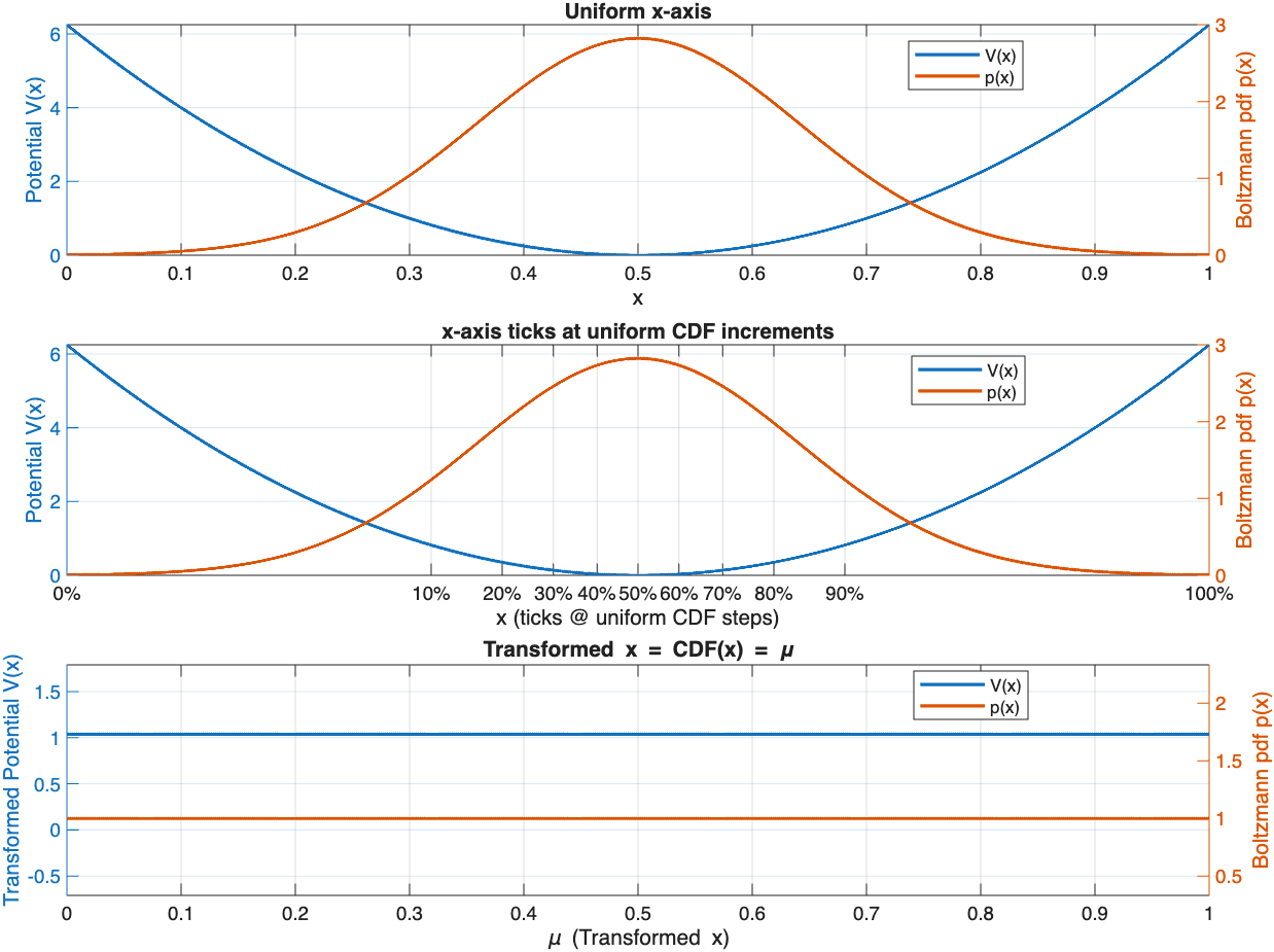
The corresponding Boltzmann distribution (for inverse temperature $\beta = 1$ here) is:

$p(x) = \frac{e^{-\beta \, V(x)}}{Z} = \frac{e^{-25\beta (x - 0.5)^2}}{Z}$

where the normalization constant $Z$ ensures $\int_0^1 p(x) \, dx = 1$:

$Z = \int_0^1 e^{-25\beta (s - 0.5)^2} \, ds$

The first subplot shows the cut-off HO potential and matching Boltzmann distribution (Gaussian).

The cumulative distribution function (CDF) is then:

$P(x) = \frac{\int_0^x e^{-25\beta (s - 0.5)^2} \, ds}{\int_0^1 e^{-25\beta (s - 0.5)^2} \, ds}$

If we define a new variable:

$\mu = P(x)$

this transformation maps $x \in [0,1]$ to $\mu \in [0,1]$.
The differential transforms as:

$d\mu = \frac{dP}{dx} \, dx = p(x) \, dx$

The second plot shows the same potential and Boltzmann distribution, but the x-axis is marked in uniform increments of the CDF measure $\mu$.

In the new coordinate $\mu$, the probability measure becomes:

$p(x) \, dx = d\mu$

which corresponds to a uniform distribution on $[0,1]$:

$p(\mu) = 1$

Using this measure, there are no potential energy gradients as every part of the distribution is equally likely. The constant offset of the energy is selected to keep the partition function constant. For more examples and details on the partition function see Additional Notes at the end of this post.

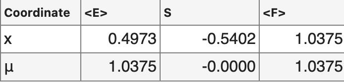Our transformation changes not only the potential and Boltzmann distribution, but also the expectation values of energy and entropy. Importantly, the free energy calculated as $F = E - T \cdot S$, stays conserved under this re-parametrization.

Takeaways

The energy and entropy of a physical system are dependent on the coordinate system are not fundamental quantities. Instead, the potential energy and entropy are a function of one's choice of coordinates. What we've done here could be called "flattening the measure" or "uniformizing the measure", or in measure theory terms we've applied a change of variables that transforms our initial measure on the x coordinate into the Lebesgue measure. More generally, we can apply any coordinate transform to the variables we measure with respect to, and we will get a new set of energy and entropy values. What remains preserved is the Free energy of the system, and notably at thermodynamical equilibrium it is exactly this quantity that is minimized. In other words, any choice of coordinates will agree on what distribution will be reached at thermodynamical equilibrium, but two coordinate systems can disagree on the contributions from energy and entropy terms.

The takeaway from this excercise is quite interesting: There is nothing special about using spatial distance or momentum coordinates to parametrize the system. Rather, we can always transform our coordinates such that we remove any potentials, and the resulting distribution becomes uniform. This process is how I understand conceptualize forces in thermodynamics, I've been feeling an uneasy suspicion towards potential energy as a concept in particular.

The way we measure potential energy is as a deviation from a uniform probability density in a Boltzmann distribution (in a constant potential the occupation probability of a state only depends on the number of degenerate states corresponding to that energy level, so if some patch of space has more particles that means there's an attractive potential there, and vice-versa for repulsion), but we never really measure potential energies, just occupation probabilities. From a descriptivist point of view when we say that two particles attract all we're saying is that they're more likely to be found close to each other than chance. In this spirit another natural description of interactions in physics is by assigning more states to a given part of the distribution or macrostate to account for the increased occupation frequency. In order to do this we need to perform a kind of coordinate transformation. We assign a larger part of the domain to regions of high probability density, and smaller parts to less probable regions, much like performing histogram equalization on an image.

To summarize: Entropy and energy are two sides of the same coin. Picking a specific coordinate system to measure in, we fix the gauge and measure a gauge-dependent entropy and energy, but always the same gauge-invariant free energy. Depending on the choice of coordinates, we can remove any entropic or energetic force from our system.

Side note: Coordinate remapping is one-to-one for all distributions

So far we have only considered what happens to the stationary, equilibrium distribution and the potential $p_*$ under these transforms. However, it is not obvious what this tranformation will do to other, non-equilibrium distributions, which will be important for exploring the temporal dynamics of the system.

We have defined the cumulative map from $x$ to $\mu$

$\mu = F(x)=\int_{a}^{x} p_*(s)\,ds\in[0,1], \qquad \frac{d\mu}{dx}= p_*(x).$

Because $p_*>0$ and integrable, $F$ is strictly monotone and hence bijective. Furthermore, this map does not bake in any particular $p(x,t)$: it is defined from $p_*$ alone. For any other evolving $p(x,t)$, we can calculate a new transformed distribution

$q(\mu,t) = \frac{p(x,t)}{p_*(x)}\quad\text{with}\quad x=F^{-1}(\mu),$

Thus $p\mapsto q$ is a one–to–one reparametrization for all distributions, not just the equilibrium.

Diffusion in transformed coordinates

Now I will examine how the diffusion equation under a potential (the Smoluchowski/Fokker–Planck equation) changes. The Smoluchowski/Fokker–Planck equation and associated probability flux are can in general be written as:

$\partial_t p(x,t)=\partial_x\!\left[D\big(\partial_x p(x,t)+\beta\,p(x,t)\,\partial_{x}U(x)\big)\right],$

$J(x,t)=-D\big(\partial_x p+\beta p\,\frac{dU}{dx}\big).$

The equation contains two terms: A diffusion term that is purely entropic in nature, and a drift term due to the energetic potential.
The unique stationary density we've been using is:

$p_* (x)=\frac{e^{-\beta U(x)}}{Z},\qquad Z=\int e^{-\beta U(x)}\,dx .$

Using the fact that: $\frac{d\mu}{dx}=p_*,$

$\partial_x=p_*\partial_\mu,$

and

$\ \frac{dp_*}{dx}=-\beta \frac{dU}{dx} p_*,$

we can write $p= p_* q$ and compute

$\partial_x p+\beta p\,\frac{dU}{dx}=\partial_x(p_* q)+\beta\,p_* q\,\frac{dU}{dx} = p_*^2\,\partial_\mu q .$

After the transformation, the flux from the Smoluchowski equation becomes

$J(x,t)=-D\,p_*^2(x)\,\partial_\mu q(\mu,t).$

Now we can insert this expression into the continuity equation $\partial_t p=-\partial_x J$, and replace $\partial_t p=p_*\,\partial_t q$ and $\partial_x=p_*\partial_\mu$ to obtain a drift-free Smoluchowski equation in $\mu$:

$\;\partial_t q(\mu,t)=\partial_\mu\!\big(D_{\rm eff}(\mu)\,\partial_\mu q(\mu,t)\big),\qquad D_{\rm eff}(\mu)=D\,p_*^2\!\big(x(\mu)\big).\;$

In this coordinate system, there is no drift term in $\mu$. All drift/bias terms have been absorbed by the coordinate change.

The stationary solution is $q_\infty(\mu) = 1$, i.e. $p_\infty=p_*$ and the equilibrium distribution matches in both coordinates.

Boundary conditions also map accordingly: reflecting/absorbing walls at $x=a, b$ become reflecting/absorbing at $\mu=F(a), F(b)$.

We can compare the evolution of the densities in the two coordinate systems, $p$ and $q$, by simulating the diffusion in a HO potential in MATLAB. Here, I'm simulating diffusion in a HO from the section on entropic forces:

$V(x) = 25(x - 0.5)^2, \qquad x \in [0,1]$

In the figure below, the left side shows the time-evolving solution to the regular Smoluchowski equation in the potential with a narrow Gaussian initialized at $x = 0.72$. The black and red lines trail the positions of the mean and mode respectively.

The right side shows the same diffusion process expressed in measure-flattening coordinates. Instead of the potential, the local effective diffusion constant $D_{eff}$ is plotted here in addition to the density.

There are two notable differences between the two: For one, the right distribution shows a splitting of the mean and mode over time. The mean quickly converges to the midpoint of the distribution, while the mode maintains its position at the rightmost edge for the duration of the simulation (in the limit of $t \rightarrow \infty$ the mode should disappear altogether, as the distribution becomes flat). This is to be expected, as our coordinate transformation is non-linear, and the shape of the distribution itself changes over time, whereas in the x-measure we maintain the Gaussian shape. The mode of a distribution is not preserved by our transformation, but the mean in fact is.

The second striking difference is in how the drift over time is achieved in both cases. In the left case, an explicit potential leads to a drift term in the Smoluchowski equation. In the right, flattened case, there is no drift term, and instead a non-homogeneous diffusion constant results in sped-up diffusion where the coordinates have been stretched, and slowed-down diffusion where they have been compressed. The variable diffusion constant leads to the afforementioned distortion of the distribution over time, and is to be expected as we set the diffusion constant to be constant in the $x$-coordinate system.

There is a third gauge we can apply that yields constant-diffusion, also called the heat gauge as it transforms the equation into the regular heat equation (see Additional Notes below). In this gauge, we would rescale the the flattened or original coordinates such that every location has uniform diffusivity, in the same way that the flattened gauge creates constant densities. They are, however, mutually exculsive and information about the initial distributions has to be contained somewhere. It can be shuffled around between non-constant potential, diffusivity and even temperature, or mixed between these.

In summary, applying a coordinate transform that re-partitions energy and entropy, the Smoluchowski equation re-partitions diffusion and drift terms. Under the transform that flattens the measure, the drift term completely vanishes, and we are left with a vanilla diffusion equation but at the cost of introducing a non-uniform diffusion constant.

Additional Comments:

More on Entropy, Energy and Coordinate Transformations

Throughout this post I’ve been treating potential energy as an expression of our choice of coordinates over probability space rather than a fundamental quantity. Here’s why I think this view hits thermodynamics more directly. The most eloquent and insightful treatment of this topic I know is from Gabriele Carcassi (link), absolutely worth checking out!

Let's look at another specific example, the Boltzmann distribution for a linear potential on $x\in[0,\infty)$.

Original coordinates:

$p_x(x)=\beta U_0\,e^{-\beta U_0 x},\qquad Z_x=\int_0^\infty e^{-\beta U_0 x}\,dx=\frac1{\beta U_0}$

where $\beta = \frac{1}{k_B ,\ T}$. We can calculate the Energy expectation value and differential Entropy for this distribution,
as well as the Helmholtz free energy and partition function through a Legendre transform from the energy:

• Energy $\langle E\rangle_x=\int_0^\infty U_0x\;p_x(x)\,dx=\frac1\beta,\quad$.

• Entropy $S_x=-\!\int_0^\infty p_x\ln p_x\,dx=1-\ln(\beta U_0)$.

• Partition function $Z_x=\int_0^\infty e^{-\beta U_0 x}\,dx=\frac1{\beta U_0}$.

• Helmholtz Free Energy $F_x=\langle E\rangle_x-TS_x = -\frac1\beta\ln Z_x = -\frac1\beta\ln\!\bigl(\tfrac1{\beta U_0}\bigr) = \frac1\beta\ln(\beta U_0)\,$.

Logarithmic coordinate transform:

Now we'll transform the x-coordinate, for example a logarithmic remapping:

$\mu=\ln\!\bigl(\frac{x}{x_0}\bigr),\quad x=x_0e^\mu,\quad \mu\in(-\infty,\infty)$

The Jacobian for this coordinate transform is $\frac{dx}{d\mu}=x_0e^\mu$. The new probability density is

$p_{\mu}(\mu) = p_x(x)\,\frac{dx}{d\mu} = \bigl(\beta U_0\,e^{-\beta U_0x}\bigr)\,(x_0e^\mu) = \beta U_0\,x_0\,e^{\mu-\beta U_0}$

$E_{\mu}(\mu)=-k_BT\ln p_{\mu}(\mu)+\text{const}=U_0x_0e^\mu-k_BT\,\mu+\text{const}.$

From this we can calculate:

• Energy $\displaystyle\langle E\rangle_{\mu} =\int p_{\mu}\,E_{\mu}\,d\mu =\langle E\rangle_x+k_BT\!\int p_{\mu}\,\mu\,d\mu =\frac1\beta+k_BT\,\langle \mu\rangle,$ so $\langle E\rangle$ shifts by $k_BT\langle \mu\rangle$.

• Entropy $\displaystyle S_{\mu}=-\!\int p_{\mu}\ln p_{\mu}\,d\mu =S_x+\int p_{\mu}\ln\frac{dx}{d\mu}\,d\mu =S_x+\langle \mu\rangle,$ so $S$ also shifts by $\langle \mu\rangle$.

• Partition function $Z_{\mu}=\int_{-\infty}^\infty e^{-\beta E_{\mu}(\mu)}\,d\mu=\int_0^\infty e^{-\beta U_0 x}\,dx=Z_x$, is unchanged.

• Helmholtz Free Energy $F_{\mu}=-\frac1\beta\ln Z_{\mu}=F_x$, is unchanged.

So while energy and entropy can be repartitioned depending on choice of coordinates,

$Z\quad\text{and}\quad F=-\frac1\beta\ln Z$

are identical in the $x$– and $\mu$–representations, and are in fact the true invariants under these kinds of coordinate transformations. This invariance and the direct convenient connection to the other more fundamental invariant, the partition function, are the main reason the Helmholtz free energy is so commonly used in statistical thermodynamics and related areas of physics.

But if entropy and energy can just be repartitioned through coordinate transformations, what's the point in doing any of these transformations to begin with? In other words, absolute entropy and energy rarely matter and $\Delta U$ and $\Delta S$ can equivalently calculated in any coordinate system, so why not just pick some arbitrary parametrizations and just stick with it? I think this question is very much analogous to the kind of gauge freedom that appears in various field theories. So while most choices of coordinates are certainly possible to use, there are some that have nicer properties than others. One such choice of gauge is one that remaps the coordinates in a way to encapsulate all forces in the Jacobian of the coordinate system. In this picture there are no forces, entropic or otherwise, acting on the particle or distribution. Every coordinate interval is equally likely and statistics fully replaces dynamics. The world view this picture provokes is one very much in line with GR, replacing potentials and forces with statistics and curved coordinates.

The refined statement looks something like this based:

For any Boltzmann–Gibbs equilibrium $p(x)$ on $\mathbb R$ or $[0,a]$, there is a unique monotonic reparametrization $\mu=F(x)$ that makes $p(\mu)$ uniform (i.e. all entropy, zero energy). This coordinate is the one in which the Gibbs–Shannon entropy is maximized under only the normalization constraint. Any residual structure lives entirely in the transformed energy $E(\mu)$, and the partition function (and therefore the free energy) stays unchanged.

The overall structure of the process, like the approach this entry:

1. Start with equilibrium density
   On some domain ($x\in[a,b]$ or $[0,\infty)$), take
   $p(x)\;\propto\;e^{-\beta E(x)}\,, \quad \beta = \frac1{k_B T}\,$

2. Compute the cumulative map
   $\mu \;=\; F(x) \;=\;\int_{a}^{x} p(s)\,ds, \qquad \mu\in[0,1]$ (or some other support).

3. Invert to the new coordinate

   $x = F^{-1}(\mu), \qquad d\mu = p(x)\,dx$

4. Write the transformed density
   $p(\mu) = p_x\bigl(F^{-1}(\mu)\bigr)\;\frac{dx}{d\mu} = 1,$

   or otherwise suitably normalized, whose Gibbs–Shannon entropy is

   $S[\mu] = -\int_0^1 1\!\cdot\!\ln1\,d\mu = 0,$

   or whatever the value is given some other support/normalization.

   The uniform distribution is the maximum entropy distribution in the sense of Jaynes' max entropy principle with the only constraint being normalization.

5. True invariants of the system are now a function of geometry only

• Partition function $Z = \int_a^b e^{-\beta E(x)}\,dx = \int_0^1 e^{-\beta E(\mu)}\,d\mu$

• Helmholtz free energy
  $F = -\frac{1}{\beta}\ln Z$

Constant-diffusion or heat gauge (Lamperti transform)

We can remove the position-dependent diffusivity by one additional coordinate transformation:

$s = s(\mu), \qquad \frac{ds}{d\mu} = \frac{1}{\sqrt{D_{\rm eff}(\mu)}} = \frac{1}{\sqrt{D}\, p_* (x(\mu))}.$

By defining:

$w(s,t) = q(\mu(s), t),$

and substituting into the drift-free equation in $\mu$,

$\partial_t q(\mu,t) = \partial_\mu \!\big(D_{\rm eff}(\mu)\, \partial_\mu q(\mu,t)\big),$

we obtain a uniform diffusion equation in the new coordinate $s$:

$\partial_t w(s,t) = D\, \partial_s^2 w(s,t)$

In this coordinate system, the dynamics reduce to the standard heat equation with constant diffusivity $D$, and all effects of the potential or entropy gradients are absorbed into the geometry of the coordinate map $s(\mu)$.

However, since this process stretches the coordinates relative to the uniform, flattened measure. Because of this the equilibrium distribution here is no longer uniform. There is no free lunch here, and one trades a flat equilibrium density but variable diffusion for a constant diffusion but curved equilibrium density.