Autocatalytic Degradation of Nitrocellulose
Nitrocellulose (NC) is a common propellant base in both civil and military applications. In the absence of sufficient stabilizer and due to aging, nitrocellulose based propellants are known to spontaneously ignite, posing a serious safety risk.
 Tianjin explosion crater from 2015. The primary cause was runaway NC degradation.
Linked here is some of my past work on analyzing NC degradation mainly based on microcalorimetry experiments, DFT computation and kinetic fitting:
The degradation process is complex, but generally understood to be mediated by an accumulation of and nitric acid as early products of degradation, leading to an autocatalytic cycle that can cause runaway self-heating at temperatures far lower than predicted using classical Frank-Kamenetskii theory for unaged NC. For this reason stabilizers like DPA or Akardites are added to scavange these autocatalytically active species, collectively referred to as in this post. Besides these stabilizers, real-world single-base NC propellants typically contain gellating agents (microcrystalline vs. gellated NC has different degradation properties), humefactants and other additives, while multi-base propellants include additional energetic materials like nitroclycerin, both further increasing the complexity of the cookoff process compared to pure NC.
 Nitrocellulose autocatalytic degradation scheme
In this blog entry I delve into the practical implications of the buildup and diffusion of as an extended Frank-Kamenetskii model. Notably, the slow buildup and release of such chemical species manifests as a thermal history effect, reducing the propellants critical temperature with prolonged aging or after exposure to elevated temperatures.
Interestingly, this model shows spikes and dynamics very reminiscent of a generalized exponential integrate-and-fire model (GEM). In particular, a fast variable that, for one range of values, exponentially decays back to baseline and above a critical threshold blows up, and a slower variable that shifts the critical point up or down. In the GEM, this shift is usually upwards, making neurons that recently spiked harder to excite, but negative in the modified Semenov model, making NC exposed to elevated tempeatures more unstable. This analogy will be especially relevant for the exploration in Nitrocellulose Degradation Part 2: Spikes from explosives to neurons.
Isothermal autocatalytic degradation
There is a lot of support for the idea of autocatalytic degradation in NC, but here I want to show an example of my own, collected in collaboration with Manfred A. Bohn. Isothermal microcalorimetry can be used in accelerated aging experiments at elevated temperature to compress the degradation process that can take years at ambient temperature to days, and measure the heat released by a sample with an accuracy on the order of nW/g.
This plot shows the heat released by a sample of an unstabilized sample of NC with 14% N at 70°C. The sample shows a long induction period, during which the heat release is relatively stable at a low level. After about day 5, the sample starts to noticably release more and more heat. In the days following the shown time frame, the heat release increases to upwards of 10,000 μW/g in a large heat release peak. Here, I want to focus on the induction period, during which the sample can be assumed to be at a constant temperature of 70°C throughout. After isolating the autocatalytic nature of the degradation, we will reintroduce sample temperature as a variable and see how autocatalysis affects runaway heating and sample stability.
Disregarding the initial dropoff in heat release, we can fit a simple autocatalytic model to this data in Matlab. Since an insignificant fraction of the nitrocellulose degrades during this time period, we can assume that the amount stays constant throughout.
A good kinetic model to use is:
Here, the heat release is assumed to be completely due to the degradation of nitrocellulose, which itself has a 0th-order term and an autocatalytic term of fittable order. is the product of the both of these pathways. Fitting the heat release in this model to the experimental data, we see good agreement between the two.
The initial value of is set to:
and the fitted parameters are after convergence are:
While redundant here, the parameter H is kept for similarity with other models and can be adjusted to match the experimenal data for H by hand and express the other parameters on a per mole basis.
Besides confirming the presence of autocatalytic dynamics, the exponent is of interest. While often modeled as equal to 1, the dynamics here are more consistent with a value of between 2 and 3. This points towards more complex internal dynamics and multiple species that react with each other during this process. One caveat to this claim is that the loss of to the environment (glass ampoule) is ignored. Gaseous can form a reservoir during the initial stages while the reaction is slow, while the loss of to the environment later becomes less important as an equilibrium between in NC and gas phase is estabilished and the reaction picks up exponentially. However, it is a certainty that a simple first-order autocatalytic reaction scheme, with or without accounting for gaseous , is insufficient to describe the full degradation dynamics of NC.
With the motivation behind introducing an autocatalytic term established, let's leave behind the isothermal case and look at the more general case where the sample is allowed to heat up relative to the environment. In the following, I will use for simplicity, which does not qualitatively change the results.
We will start by introducing the canonical Frank-Kamenetskii and Semenov models, then modify them to include the autocatalytic term and explore its implications. Models of this nature have been introduced and analyzed by Merzhanov (1958) and El-Sayed (2003), but are unfortunately very technical.
Vanilla Frank-Kamenetskii equations
Simplifying assumptions
Modeling the full cookoff of NC is highly complex, since sample inhomogeneities, transport processes, deformation, presence of oxygen, water and impurities and other parameters need to be taken into account. This and the subsequent models ignore these for the sake of intuitive interpretability.
Additional assumptions are:
- No mass loss in early stages and constant amount of source material.
- No internal convection.
- Constant thermal properties.
- Reaction rate depends only on temperature.
- Geometry fixed and homogeneous.
The classical model assumes either fixed boundary temperature (Dirichlet) or convective heat loss (Robin). Here, we will use the convective heat loss at the surface, while the isothermal case above would be better suited to be treated with a fixed boundary temperature.
Reaction–diffusion model
In its classical form, the Frank–Kamenetskii model assumes a single irreversible Arrhenius reaction with constant material properties and heat removal by conduction only. Let denote temperature. The energy balance reads
where is density, heat capacity, thermal conductivity, reaction enthalpy per unit mass, the pre-exponential factor, and the activation energy.
Under the Frank–Kamenetskii approximation, assuming and expanding around an ambient temperature , define the dimensionless temperature
The Arrhenius term reduces to
After non-dimensionalization with characteristic length and time (thermal diffusivity ), one obtains
where the Frank–Kamenetskii parameter is
Thermal runaway corresponds to the absence of a bounded steady solution. This solution can be found by solving the non-linear Gelfand equation, if such a solution exists:
Linearizing around a steady state with perturbation :
This yields the eigenvalue problem
Instability occurs when the principal eigenvalue crosses zero. In extended geometries, the critical depends on geometry through the lowest Laplacian eigenvalue. Runaway corresponds to the loss of a bounded steady state via saddle–node bifurcation.
Sample size is included in the Frank–Kamenetskii parameter . For larger samples the exponential term tends to dominate at lower , so that larger samples tend to be more prone to runaway self heating and have a lower critical environment temperature.
The behavior of this model is still complex, and general statements are difficult to make since sample geometry is a major factor. In particular, the critical is not a single value; rather, there is a critical for each point in the sample (with the exception of some specific idealized geometries). For better tractability, we will lump the whole sample into a single point in the next section, assuming constant temperature (and in the modified model later constant ) throughout .
Vanilla Semenov (lumped) model
The lumped version of Frank-Kamenetskii, called the Semenov model, reduces the full reaction–diffusion problem to a single nonlinear ordinary differential equation with uniform temperature and reaction rates. Since the dependence on geometry is removed, this model is much more tractable. We can then reapply the intuition gleaned from this simpler model to the extended Frank–Kamenetskii model. The equation describing the Semenov model is
Here, combined are a heat transfer coefficient per unit heat capacity at the sample surface.
Non-dimensionalizing this equation, we are left with an equation that governs the whole sample this time:
which expresses a competition between exponentially growing heat generation and linear heat loss.
Steady states satisfy
Graphically, this corresponds to the intersection of:
- the heat generation curve ,
- the heat loss line .
The following animation shows plots the solutions as the control parameter is varied continuously. This parameter represents the relative strength of heat removal compared to heat production.
For large (strong cooling), the linear heat-loss curve is steep and intersects the exponential twice:
- a lower-temperature stable fixed point (blue, filled)
- a higher-temperature unstable fixed point (red, open)
Small perturbations away from a stable fixed point exponentially decay, while perturbations away from an unstable fixed point exponentially grow. For temperatures higher than the unstable fixed point the temperature exponentially increases in runaway self-heating. Writing
the derivative at a fixed point is
Hence:
- : stable,
- : unstable.
At the critical value
the two fixed points collide and annihilate in a saddle–node bifurcation (black marker). Beyond this point, no steady state exists: heat generation exceeds heat removal for all , and the system undergoes thermal runaway at any temperature.
The right panel accumulates the fixed points as varies, revealing the characteristic fold structure of a saddle–node bifurcation. The vertical line indicates the current parameter value corresponding to the intersection picture in the left panel.
Importantly, ignition is not a gradual loss of linear stability in the Semenov model (and by extension the Frank–Kamenetskii model). Instead, it is a structural loss of equilibria: the stable branch disappears entirely. This geometric viewpoint generalizes directly to the next model, where the additional presence of the variable shifts the underlying bifurcation structure.
Semenov model with autocatalysis
Extended reaction system
To include the effect of in this model, we use the following scheme:
Here, I assume first-order autocatalytic dynamics and the same activation energy and heat release from both the regular and the autocatalytic pathways. is produced in a temperature-dependent manner, and lost at the surface to the environment at a rate proportional to . The variable could be used to model a reservoir of in the environment, even with its own dynamics, but is set to 0 in the following sections.
After some simplification and combining parameters, we get these two equations:
These are the equations used in the next sections.
Stability analysis
To understand what effect introducing has on the dynamics, let's first look at the intersections between the heat production and heat loss curves for different values of , keeping all other values constant:
has a near-multiplicative effect on the heat production curve, making it appear to shift to the left as increases. For high enough values of , any value of will lose its fixed points and always undergo runaway heating. To illustrate this, we draw a phase diagram by scanning through a grid of combinations of and . We can see a clear boundary of stability between regions of instability and stability:
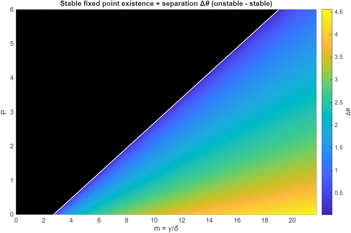 In this plot, the black region indicates unstable parameter combinations. Where there are fixed points,
the parula color map indicates how far the fixed points are apart. Near the boundary between the stable and unstable region, the separation between
the fixed points tends to 0, as is expected from a saddle-node bifurcation.
In this plot, the black region indicates unstable parameter combinations. Where there are fixed points,
the parula color map indicates how far the fixed points are apart. Near the boundary between the stable and unstable region, the separation between
the fixed points tends to 0, as is expected from a saddle-node bifurcation.
Since high brings the system closer and closer to the unstable region, it is apparent that autocatalytic dynamics have a compounding effect on instability. As the temperature grows, so does the production rate of , which in turn increases the rate of temperature growth.
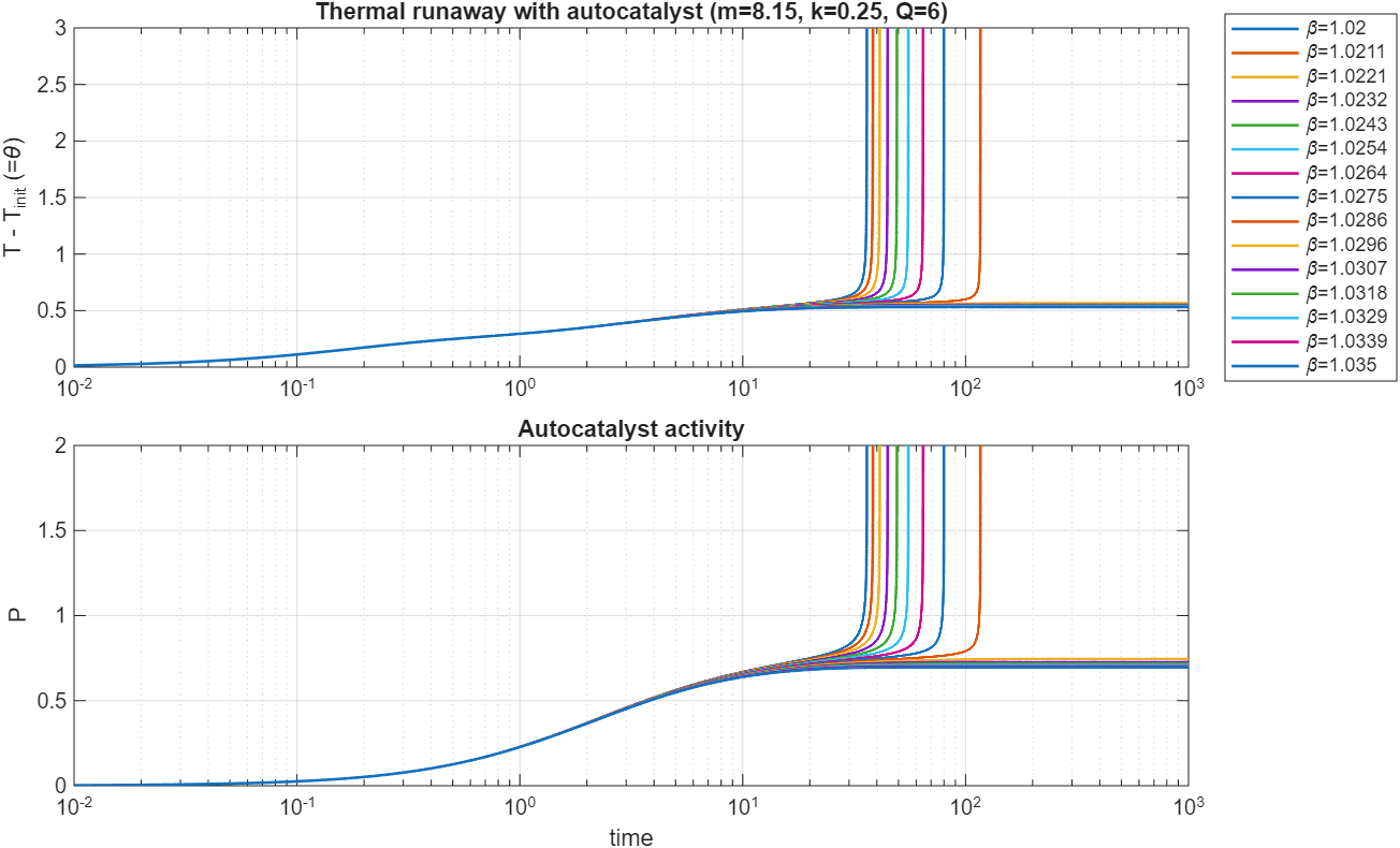
By simulating the dynamics for specific values of (called in the plots below), (called in the plots below) and , and setting , we can observe the dynamics of and . Varying the loss rate , we see another clear boundary between stable and unstable conditions:
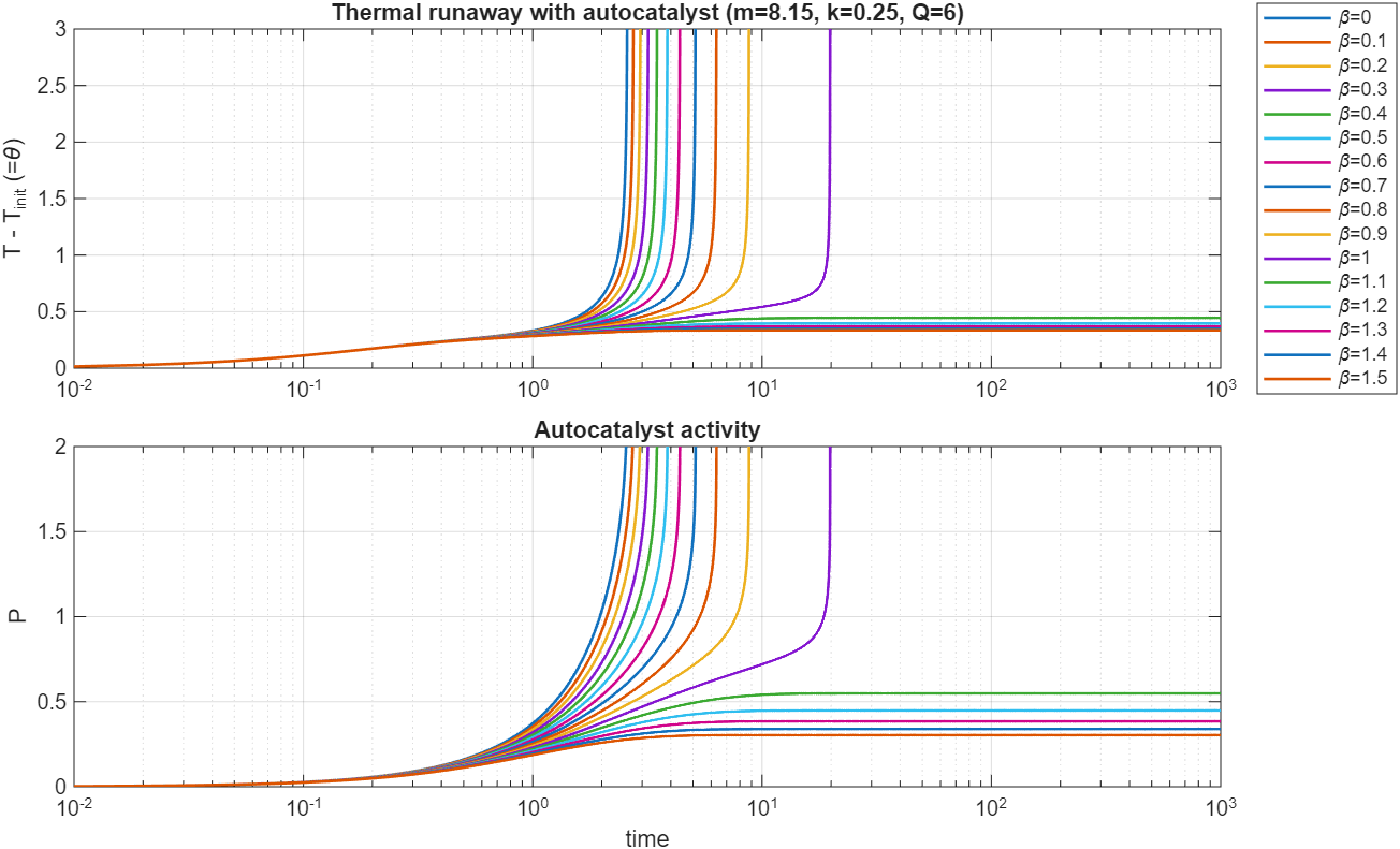
Similar to the vanilla Semenov model, the transition between stability and instability is abrupt. Running a second scan of over a much more narrow range of parameters, we see this distinction between two families of curves very clearly:
We can similarly plot a phase digram over combinations of parameters (divided by here) and :
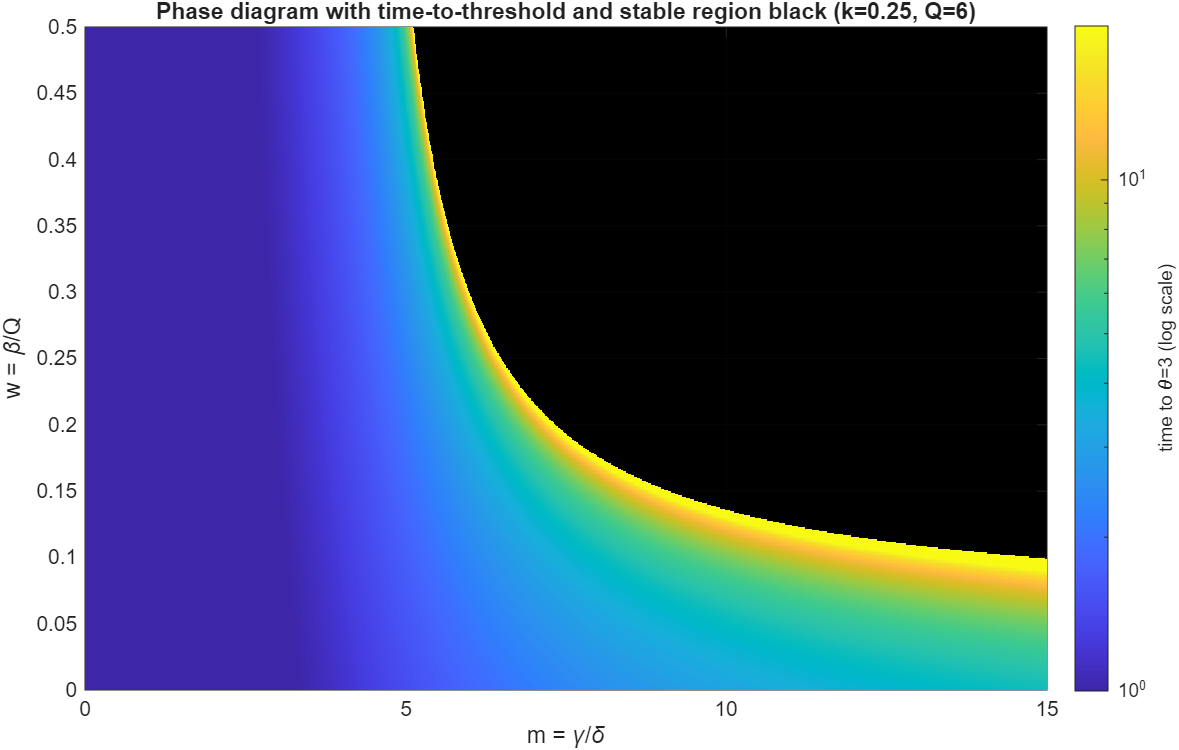
The black region indicates indefinite stability, while the parula colormap encodes the time until reaches a threshold value of 3. Notably, while both and play a role in controlling stability, the heat dissipation term in the form of is much more important as the heating rate increases exponentially faster with respect to , but only linearly or at most with a polynomial dependence with .
For a mathematically rigurous stability analysis, consult Merzhanov (1958) and El-Sayed (2003).
Memory effect: Thermal history dependence of stability
The most striking change that autocatalytic introduces to NC degradation is its role as a kind of memory. In the regime where loss of is much faster than that of heat, it acts as a kind of integrator over the thermal history of the sample. This is a good assumption for small samples that cool out quickly, while is much slower to diffuse out of the NC matrix. As the sample is heated and is released, it build up and comparatively slowly decays back to baseline over time once the sample is cooled back down.
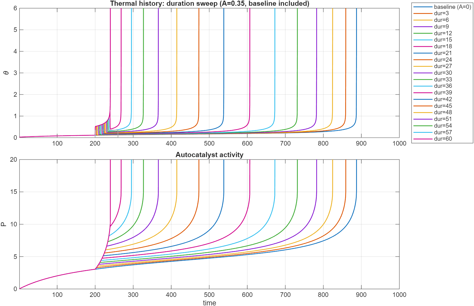
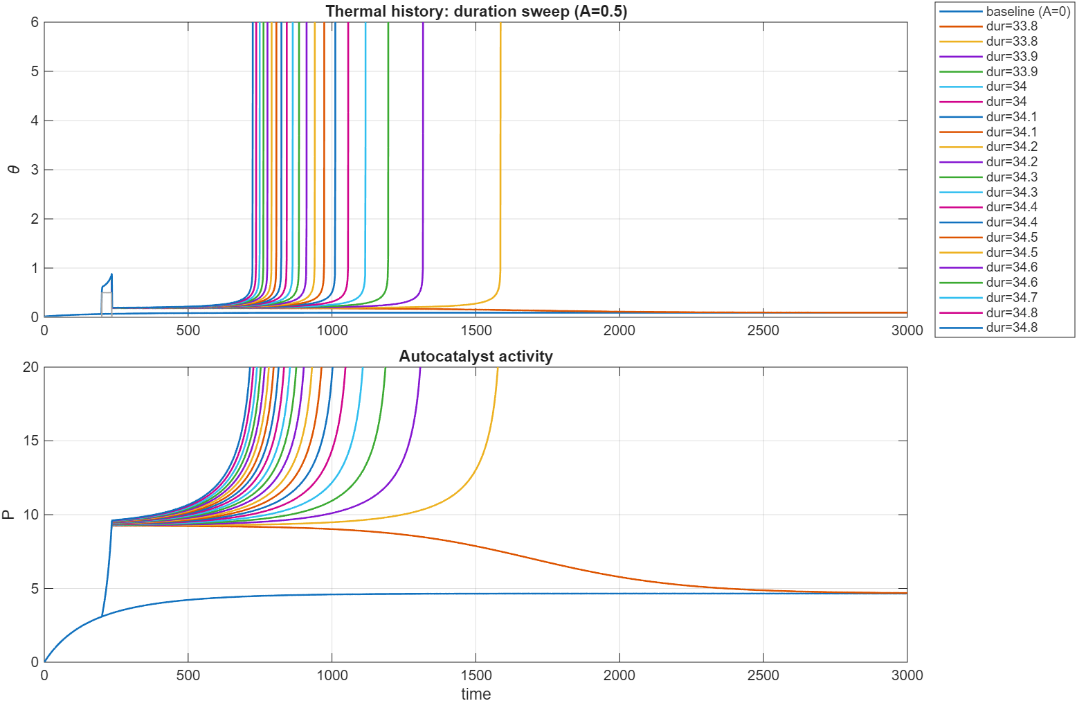
To visualize this point, we can run a simulation with these parameters: , , (called Q below), . Note how , the decay rate of is much slower than that of temperature, . The system is heated up for a short time by exposing it to an elevated .
Here is a plot of the dynamics of and over time for step of fixed amplitude for variable duration. For these parameter ranges the sample is supercritical and will always reach thermal runoff, even for no step-up in temperature, but the time until runoff drastically varies depending on the duration of the step:
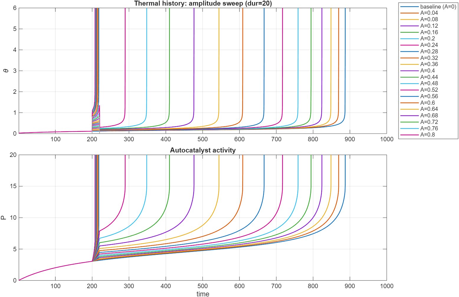
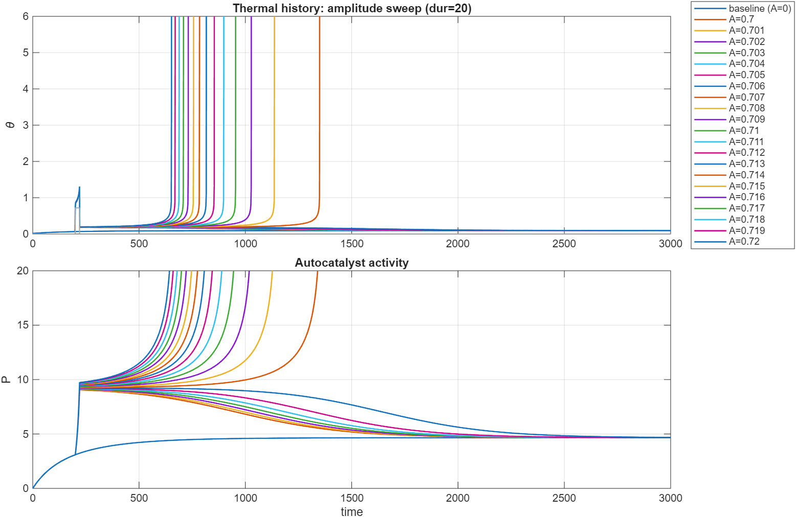
Similarly, this plot shows the same variables for a step of a fixed duration of , but the amplitude is varied (called A here).
The result is similar to that above. In both cases, after the exposure the sample returns to a temperature practically indistinguishable from baseline, before
showing runoff unexpectedly early.
This is similarly reproducible for systems that are subcritical. In this case, a short exposure to elevated temperatures can tip the system towards criticality, an important detail to know when handling these substances. Similar to the canonical equations, the system shows a clear distinction between two families of curves with a sharp cutoff.
Changing two of the parameters, , , (called Q below), , we are in a subcritical regime. Heating the sample up
with a fixed and variable , we get this plot. Note the very narrow range of parameters scanned here.
Similar results for a fixed , variable . The variation of the temperature is only on the order of , clearly highlighting the
sharp distinction between subcritical and supercritical solutions.
Frank-Kamenetskii with autocatalysis
We could similarly write out the equations for an autocatalytic Frank–Kamenetskii model. However, I do not see a clear motivation for this in order to gain intuitions for this model that cannot be obeserved in the lumped model.
Instead a couple comments:
-
In an extended sample with slow diffusion, the effect of memory is exacerbated. For a granule that is exposed to an elevated temperature, we expect a gradient of from the center, dropping off outward towards the surface, where is released. While little or barely increased can be observed at the surface, while the center of the granule is starting to strongly decompose and close to runoff. This effect would also be seen for a sample heated up locally at the surface, with heat and diffusing towards the center where loss is less important. Some comparisons for films of NC (like that used for movies) vs. granules might be interesting.
-
If we map our Semenov model onto a single neuron as mentioned as described at the beginning, then the extended Frank–Kamenetskii model best maps onto an excitable medium. Such media can support fascinating dynamics, such as Turing patterns, topological action potentials or Fisher waves. While the Semenov model lacks the necessary complexity to allow for a return to baseline, it might be possible to see thermokinetic oscillation. I have not thought about this deeply enough so far, so I cannot affirm of disprove this possibility at the moment.
Issues with these models for NC degradation
There are multiple assumptions in these models that differ from real NC, besides the simplifications regarding homogeneity, convective heat loss and no physical deformation mentioned here.
For one, the kinetic order observed for real samples of NC is not 1, rather closer to 2.5. While that does not significantly change the qualitative behavior of these equations, it points towards a much more involved mechanism, rather than simple first order autocatalysis. In particular, if the reaction order of 2.5 in the isothermal microcalorimetry experiment is to be believed, there are multiple hypotheses to address it:
- Dead space in ampoule in ampoule acts as a slowly filling reservoir of
- Higher order autocatalysis (>3) is happening at the same time
- Fast equilibrium depleting in one of its forms is present, alongside a second order degradation reaction (this can give a bona fide order 2.5 mechanism)
More on this in the next blog entry.
Literature Overview and Notes:
-
Thermal hazard evaluation on spontaneous combustion characteristics of nitrocellulose solution under different atmospheric conditions cites ~12.6% N as threshold?
-
Comparisons of TGA and DSC approaches to evaluate nitrocellulose thermal degradation energy and stabilizer efficiencies compares low-N (11.71%) vs high-N (13.47–13.57%)
-
Stability Predictions for the Autocatalytic Decomposition of Nitrocellulose in Toluene
-
Spontaneous Ignition Behavior of Nitrocellulose–Sulfuric Acid Mixtures
-
Effect of porous magnesium oxide as a stabilizer for nitrocellulose
-
Experimental Study on the Fire Properties of Nitrocellulose with Different Structures
-
Study on the effect of ethanol content on the fire risk of nitrocellulose Samples with higher surface area ignite easier, should be opposite assuming offgassing main break? However, iPrOH! Same group: Study on the effect of ethanol content on the fire risk of nitrocellulose
-
Essential hazard assessment of nitrocellulose via numerical and experimental investigation and calorimetry thermokinetic approaches EtOH shows little effect… Missing pure NC, take into account heat capacity of EtOH? Essential hazard assessment of nitrocellulose via numerical and experimental investigation and calorimetry thermokinetic approaches
-
Stabilizers for Nitrocellulose‑Based Propellants: Insights from Compatibility and Thermal Stability
-
Estimation on the Safe Storage Temperature of Nitrocellulose with Different Humectants
-
A Simplified Method to Predict the Heat Release Rate of Industrial Nitrocellulose Materials Oscillation in mass loss rate, or noise?
-
thermal reaction–diffusion (cookoff / thermal explosion)
-
Frank-Kamenetskii 1938 Wikipedia Grokipedia
-
On the stationary theory for heat balance of powder and explosive condensed phases (1961)
-
A review of one aspect of the thermal-explosion theory (2006)
-
Model with memory. Induction time. Analogous to adexp model w/ P slow variable? Alternatively, excitable medium → Fisher waves, boundaries, etc.
-
Chemical reaction modeling of industrial scale nitrocellulose production for military applications Reaction diffusion model of nitrocellulose synthesis, values for diffusion coefficients, fiber lengths, etc