This post belongs to a three part series containing:

• Entropic Gravity Part 1: Coordinate remappings and entropic forces
• Entropic Gravity Part 2: Parameter choice and randomness
• Entropic Gravity Part 3: Diffusion in non-uniform time and space

Diffusion in non-uniform time and space

In this blog post I want to tie together the previous two and apply the coordinate transformations discussed there to Einsteinian gravity, General relativity (GR). At its core, GR replaces Newtonian gravitational potentials with coordinate remappings, making it a suitable playground for exploring if gravity can be equivalently thought of as an entropic phenomenon for diffusion.

There are three contributions:

• Space stretching
• Time dilation
• Temperature gradients

Classical Diffusion in inhomogeneous Space

One of the effects of GR is that the geometry itself changes the "density" of space, even before introducing any explicit forces. In particular, when measuring the volume of space around massive object, it is stretched, i.e. summing up all spatial volume elements gives a larger volume than would be expected with a naive $V = \frac{4}{3} \pi r^3$ calculation.

In 1D, if the proper distance is

then the coordinate $x$ does not measure physical distance uniformly. A coordinate interval $dx$ in a region with larger $\sigma(x)$ corresponds to a larger amount of proper space.

If diffusion is unbiased in proper space, then the stationary density is uniform with respect to $ds$, not with respect to $dx$. Writing

and taking $\rho_{\text{proper}}(s)=\text{const}$, we get

So a region where space is stretched ($\sigma > 1$) collects proportionally more probability mass, while a compressed region ($\sigma < 1$) gets proportionally less. The reason is purely geometric: there is simply more proper space packed into the same coordinate interval.

Equivalently,

In higher dimensions, the same idea is expressed by the spatial part of the metric $h_{ij}(x)$. The proper volume element is

so diffusion that is uniform in proper space has stationary coordinate-space density

This is the multidimensional version of the 1D stretch factor. If space is stretched isotropically by a factor $\sigma$ in each direction, then

so the equilibrium density in coordinates is enhanced by the same cubic factor. In this sense, curvature can bias diffusion purely through the local density of available spatial states.

Classical Diffusion in inhomogeneous Time

One of the consequences of GR is gravitational time dilation (for a refresher watch Interstellar, it's a good movie), i.e. time runs slower near massive objects. Outside of a spherical mass, the local rate of the flow of time goes like $\frac{dt}{d\tau} = \sqrt{1 - \frac{2 \cdot G \cdot M}{r c^2}}$, leading to a rate of flow of time dependent on the radial distance. This is what I'm going to build towards, but first we should build some intuition on some simple examples.

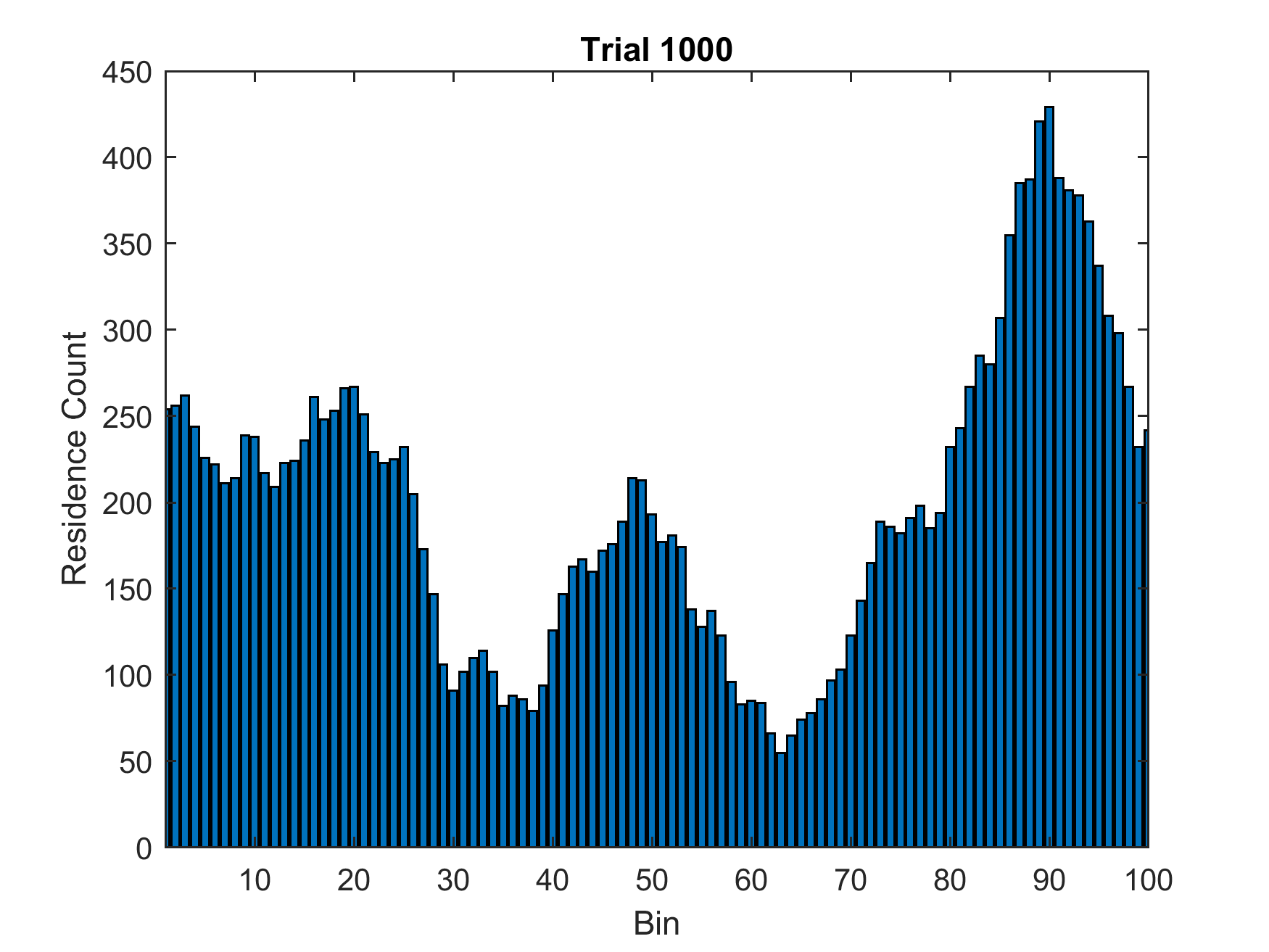
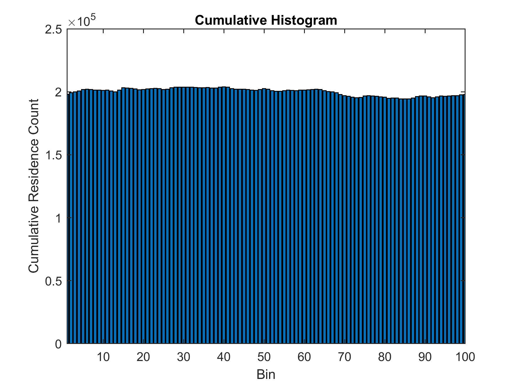
First, let's explore what effect different rates of flow of time have on a particle diffusing on a 1D ring. As a baseline, here's simple Monte-Carlo simulation using an unbiased random walk with homogeneous time flow in MATLAB (20000 time steps per trial, 1000 trials) and plotting the histogram of where the particle is located at each step shows the expected uniform distribution.

So what effect do variations in the flow of time have on diffusing particles? To make the flow of time inhomogeneous, I picked the first 10 bins on the ring and made the random walk in that region only update once for every two updates on the rest of the ring. Running the same Monte-Carlo simulation now yields a different result: The particle on average spends twice as much time in the region with slowed time.

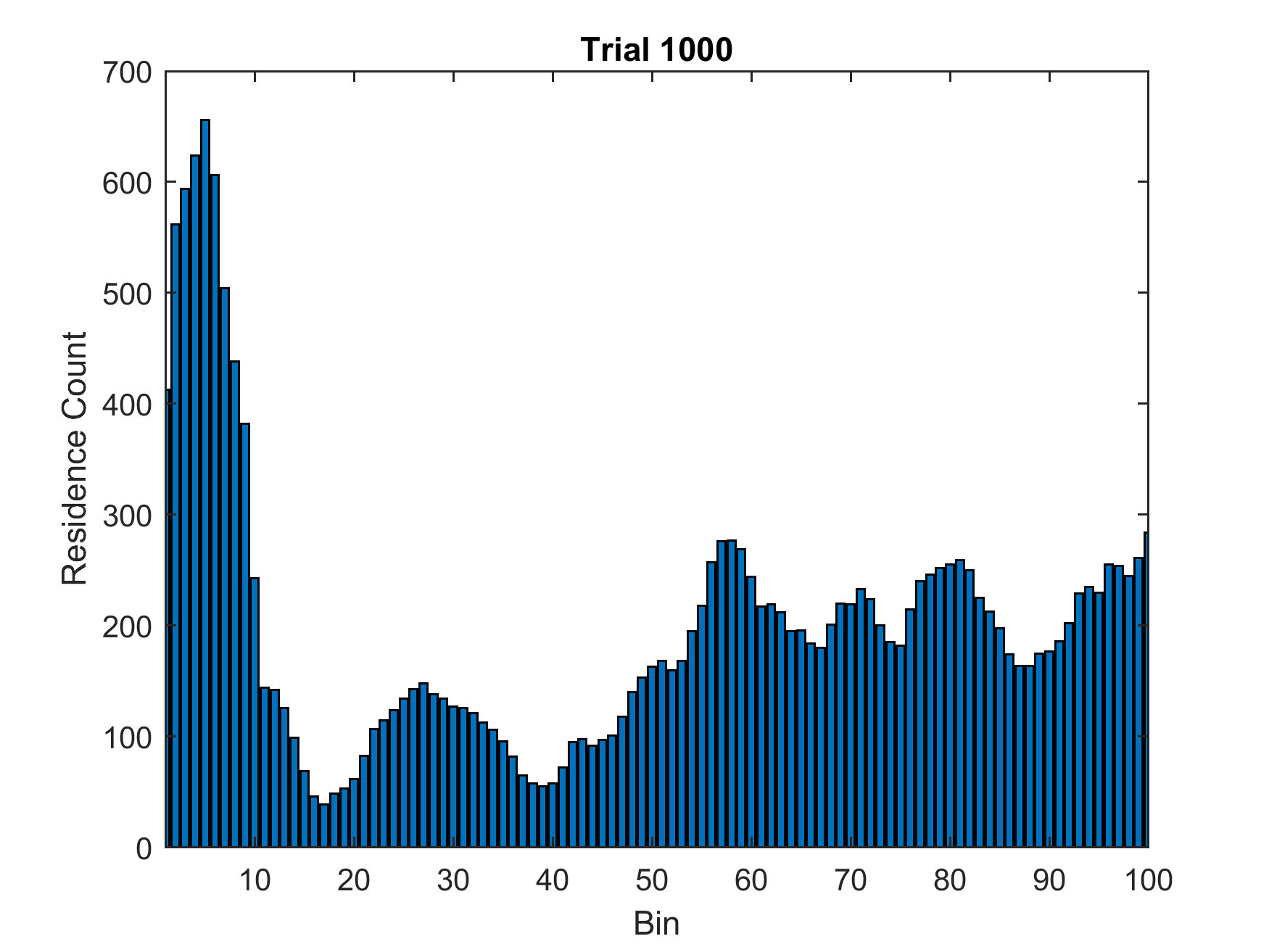
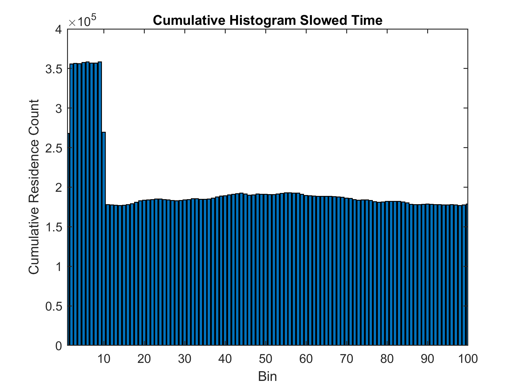
This simulation can be run with many different amounts of time dilation (or time-dilation factors), but it always yields the same result:
The probability of finding a particle in a bin with slowed time relative to a bin outside that region is directly proportional to the amout of time dilation, so let's try to generalize this point. We can add the effect of time dilation to the Fokker-Planck equation for diffusion by using the chain rule on coordinate time (local flow of time) and use proper time instead, or by incorporating the slower rate of passage of time into the diffusion constant. I will use the latter approach.

We start from the usual one-dimensional Fokker–Planck equation written in proper time (the particle’s own clock, wherever it is):

$\frac{\partial p}{\partial \tau}(x,\tau) = D_0\,\frac{\partial^2 p}{\partial x^2}(x,\tau)$

The outside world measures coordinate time $t$. The two clocks are linked by the time-dilation factor:

$\alpha(x) = \frac{dt}{d\tau}(x) > 1$

Or alternatively:

$d\tau = \frac{dt}{\alpha(x)}$

Because $\tau$ advances more slowly where $\alpha(x)$ is large, the effective diffusion coefficient seen in coordinate time is:

$D(x) = D_0\,\frac{d\tau}{dt} = \frac{D_0}{\alpha(x)}$

Replacing $D_0$ with $D(x)$ gives the Fokker–Planck equation in coordinate time:

$\frac{\partial p}{\partial t}(x,t) = \frac{\partial^2}{\partial x^2} \left[ D(x)\,p(x,t) \right]$

In equilibrium, $\frac{\partial p}{\partial t} = 0$, so the equation becomes:

$\frac{\partial^2}{\partial x^2} \left[ D(x)\,p_{\text{stat}}(x) \right] = 0$

Integrating twice (and assuming reflecting boundaries so the net probability flux is zero) gives:

$D(x)\,p_{\text{stat}}(x) = \text{const}$

Substituting $D(x) = \frac{D_0}{\alpha(x)}$ gives the final result:

$p_{\text{stat}}(x)\,\alpha(x) = \text{const}$

Or in other words:

$\frac{p_{\text{stat}}(x)}{\text{time-slow-down factor}} = \text{const}$

This is a general statement of what the earlier Matlab simulations showed, namely that regions with slowed time lead to a higher probability of finding a particle inside.

From a classical thermodynamical perspective, we could interpret this result as stemming from a potential that attracts the particle to this region. Adding this potential to a Fokker-Planck equation (commonly called the Smoluchowski equation in this form) with homogeneous flow of time gives us:

$\frac{dp}{dt} = D\left( \frac{d^2p}{dx^2} + \frac{d}{dx} \left( \frac{p}{k_B T} \frac{dU}{dx} \right) \right)$

$\frac{dp}{dx} = - \frac{1}{k_B T}\,p\,\frac{dU}{dx}$ for the stationary distribution.

The potential that fulfills this condition can be found by integrating both sides:

$\int \frac{1}{p}\,dp = -\,\frac{1}{k_B T} \int \frac{dU}{dx}\,dx$

$\ln p = -\,\frac{1}{k_B T}\,U(x) + \text{const}$

Exponentiating and plugging in the partition function for the constant of integration leads to the standard form of the Boltzmann distribution in this choice of coordinates: $p(x)\;=\;\frac{1}{Z}\,e^{-\,\frac{U(x)}{k_B T}}$

And we get an expression for the apparent entropic potential energy as a function of $\alpha(x)$:

$U(x)=k_B T\,\ln\!\bigl(\tfrac{dt(x)}{d\tau}\bigr)+C = k_B T\,\ln\!\bigl(\alpha(x)\bigr)+C .$

So what looks like diffusion or a random walk in one set of coordinates (using local proper time everywhere) is consistent with an entropic force and associated potential in another set of coordinates (using the same coordinate time everywhere).

Classical Diffusion under inhomogeneous temperature

Due to the gravitational redshift induced by a massive object, there the equilibrium temperature is not constant in GR. Instead, the Tolman–Ehrenfest effect makes it so the temperature is higher near the massive object than farther away. For a more in-detail description, see Notes on Temperature in GR below.

The Tolman–Ehrenfest relation states that

where $N(x)=\sqrt{-g_{00}(x)}$ is the lapse and $T_\infty$ is the temperature measured at infinity. Since $N(x)$ is smaller closer to a massive body, the local equilibrium temperature $T(x)$ is higher there.

There are two separate ways temperature could affect the dynamics:

1. Through the diffusion constant $D(x) = \mu k_B T$ using the Einstein equation for diffusion
2. Through the local thermally accessible state density $Z_p(x)$

The diffusion constant controls how fast probability redistributes, but not what equilibrium it approaches.

By contrast, $Z_p(x)$ determines the stationary distribution itself. Since the evolution is written in the form

any positive $D(x)$ gives the same zero-flux equilibrium condition

Therefore, $D(x)$ controls rate of approach to equilibrium, while $Z_p(x)$ controls where equilibrium density accumulates.

In the simulation below, I set up diffusion with a constant $D(x) = D_0$ and a temperature gradient. Temperautre here only acts through the local thermally accessible density of momentum states. At each position $x$, the local momentum partition factor is

For the exact 1D relativistic case used in the code,

where $K_1$ is a modified Bessel function of the second kind. This quantity measures the Boltzmann-weighted density of thermally accessible momentum states. Where $T(x)$ is larger, more momentum states are appreciably occupied, so $Z_p(x)$ is larger.

The diffusion equation solved in the Matlab script is

Equivalently, in flux form,

with reflecting boundaries.

This construction is chosen so that the stationary no-flux solution is

So the temperature gradient enters the equilibrium density through $Z_p(x)$: hotter regions have a larger thermally accessible momentum-state volume, and therefore a larger equilibrium probability density.

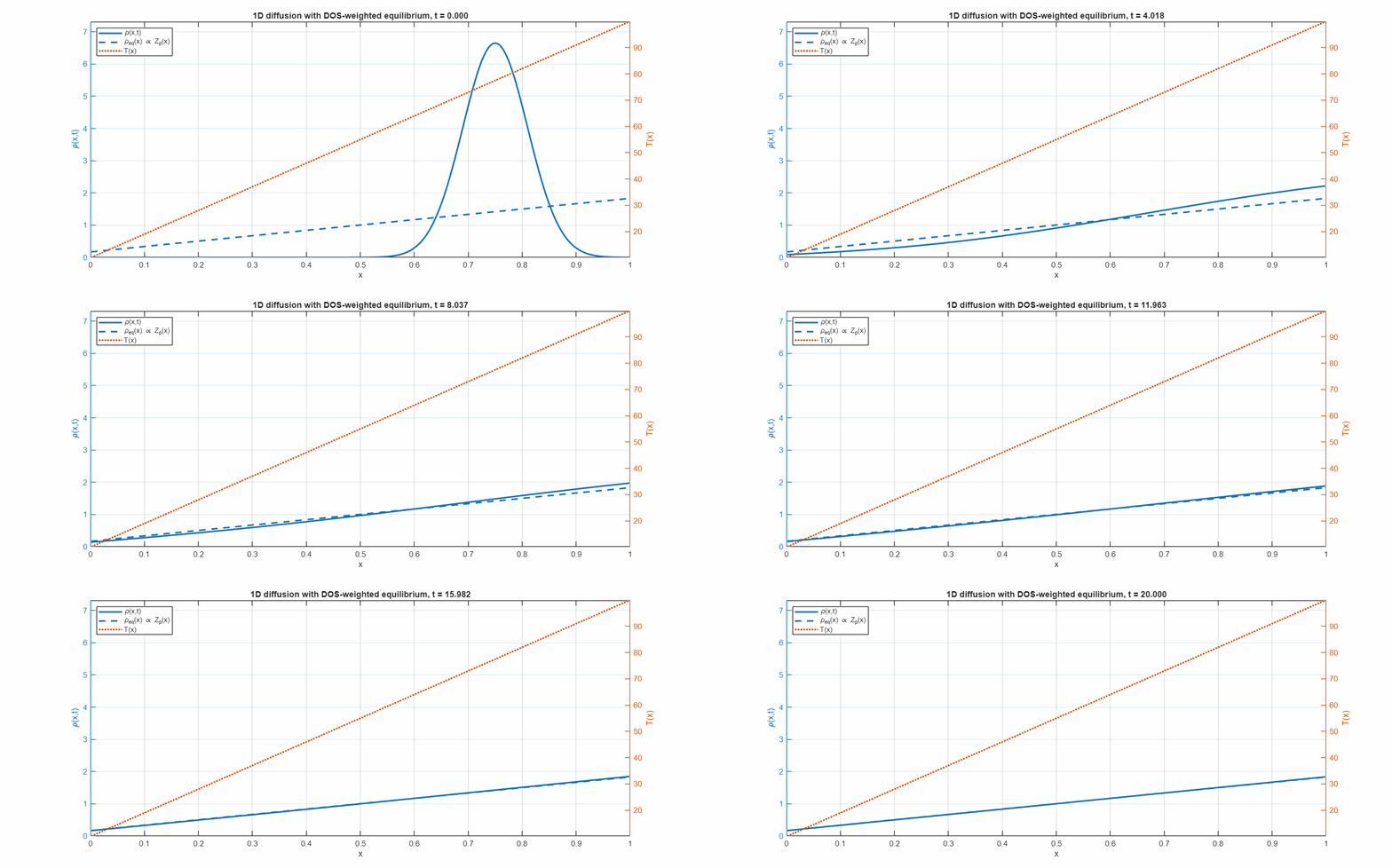
Geometric interpretation: increased available state density at higher temperature

The clean geometric reading is that temperature changes the number of momentum states that are thermally accessible at each spatial point. In 1D, the equilibrium measure can be written as

So the effective local density of available states per coordinate interval is

In the exact relativistic model,

Thus, as $T(x)$ increases, the local thermally accessible momentum-space volume increases, and the equilibrium density accumulates accordingly.

In the nonrelativistic limit, this becomes

or, if only the kinetic accessibility is retained,

So the geometrically interpreted increase in available state density with temperature is:

• higher $T(x)$ means a broader thermally occupied momentum space
• broader occupied momentum space means a larger local partition volume $Z_p(x)$
• larger $Z_p(x)$ means more equilibrium weight assigned to that position

In GR language, using the Tolman relation,

So regions deeper in the gravitational field, where $N(x)$ is smaller and $T(x)$ is higher, can be interpreted as regions with a larger local thermally accessible density of states.

Exact equilibrium density for diffusion around a massive body in GR

For a static spacetime, write the metric as

The invariant one-particle phase-space measure on the mass shell is

or, after restricting to a constant-$t$ slice,

In a static spacetime there is a timelike Killing vector $\xi^\mu = (\partial_t)^\mu$, so the conserved energy is

Thermal equilibrium is controlled by the temperature measured at infinity, $T_\infty$, and the local temperature satisfies the Tolman relation

The exact classical equilibrium distribution is then

Equivalently, using the local energy measured by static observers,

so

This is the Maxwell–Jüttner distribution in a static gravitational field.

To obtain the equilibrium density in position space, integrate over local momenta:

The momentum integral can be evaluated exactly:

so the exact equilibrium measure is

up to an overall constant factor depending only on $m$.

The main takeaway here is that we need to include the momentum part of the state density when thinking about flattening our measure later (which was not the case previously, as everything took place at the same temperature, thus same momentum states available). Furthermore, the increased temperature near our massive object leads to an increased probability of finding a particle there.

Geometric interpretation of diffusion in GR

As we just derived:

This formula actually expresses the full equilibrium bias geometrically:

• $\sqrt{h(\mathbf{x})}\,d^3x$ is the proper spatial density of states
• $N(\mathbf{x})$ sets the gravitational redshift
• the Tolman law turns that redshift into a local equilibrium temperature
• the Bessel-function factor is the exact local thermally accessible momentum-state volume

For a Schwarzschild exterior metric,

we have

Therefore

After integrating over angles, the radial equilibrium density per coordinate interval $dr$ is

In the weak-field, nonrelativistic limit,

and this reduces to the familiar barometric form

So the exact GR equilibrium density can be understood as a product of proper spatial volume and the local thermally weighted momentum-space density of states, with the Tolman relation encoding how gravity reshapes thermal accessibility.

Diffusion under a Schwarzschild Metric (unfinished)

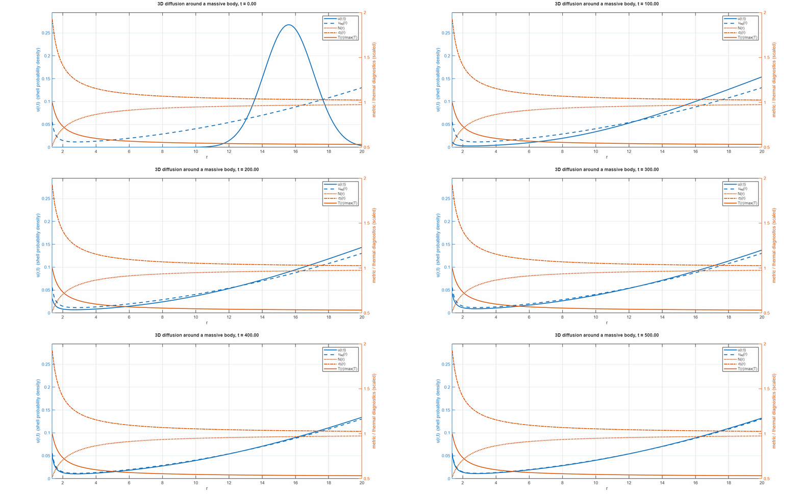
Additional Comments:

Notes on Temperature in GR

While writing this post I learned something very interesting about temperature in GR: temperature actually becomes observer-dependent due to differences in the local flow of time. Let's look at two observers, $A$ and $B$. $A$ sits far away from a massive object, where proper time aligns with coordinate time ($\alpha = \frac{dt}{d\tau} = 1$). $B$ is located much closer to the object with $\alpha > 1$. At thermal equilibrium the flux of blackbody radiation from $B$ traveling to $A$ will exactly balance out with the flux from $A$ to $B$.

However, photons energies going from $B$ to $A$ are redshifted by a factor $\frac{1}{\alpha}$ and their emission rates (per $A$'s coordinate time) appear decreased by $\frac{1}{\alpha}$. In total the observed power at $A$ is reduced $\frac{1}{\alpha^2}$ and redshifted. The reverse is true for photons going from $A$ to $B$: from $B$'s perspective energies are blueshifted by $\alpha$ and emission rates are increased by $\alpha$.

Now suppose B's local temperature is fixed at $T_B$. The power emitted locally from his frame is:

If $A$ and $B$ are at the same temperature $T$, the ratio of energy flux $\Phi_{AB}$ over $\Phi_{BA}$ would be

$\frac{\Phi_{AB}}{\Phi_{BA}} = \alpha^4$

This means they're not in thermal equilibrium as there is a net energy flux.
To achieve equilibrium, each region must have a temperature such that the flux is equal. As radiated blackbody power follows the Stefan-Boltzmann law $\Phi_{AB} = \sigma T_{A}^4$ and $\Phi_{BA} = \sigma T_{B}^4$, there must be a temperature gradient:

$\Phi_{AB} = \sigma \, \alpha^4 \, T_A^4 \stackrel{!}{=} \sigma \, T_B^4 = \Phi_{BA}$

This means $B$'s absolute temperature must be higher than $A$'s: $\, \, T_B = T_A\, \alpha$. What we've derived here is the Ehrenfest–Tolman law, which in general can be written in terms of the space-time metric $g$:

$T(x) \cdot \sqrt{-g_{00}(x)} = \text{const}$

or

$T(x) = T_\infty \cdot \alpha(x)$

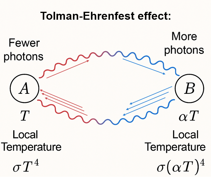
$T_\infty \cdot \alpha(x)$ is called also the redshifted temperature. So in simple words, $A$ and $B$ are at different temperatures to compensate for photon energy shifts and differences in emission rates due to time dilation.

In the Fokker–Planck equation from earlier we've ignored this effect. What we wrote was:

$\frac{\partial p}{\partial t}(x,t) = \frac{\partial^2}{\partial x^2} \left[ D(x)\,p(x,t) \right]$ and $D(x) = \frac{D_0}{\alpha(x)}$

However, our formulation of including time dilation in the diffusion constant turns out to be equivalent, which we can see by relating the diffusion constant to the local temperature using the Stokes-Einstein relation:

$D(x) = \frac{k_B T(x)}{6\pi \eta R} = \frac{k_B T_\infty}{6\pi \eta R} \cdot \alpha(x) = D_0 \cdot \alpha(x)$

Why would Entropy be Affected by Time Dilation?

While I think the fact that regions of stretched space have higher entropy per unit coordinate length as seen from afar (more states per unit length or volume than expected) is fairly intuitive, since we're used to thinking of entropy being proportional to volume as an extensive property. But why would entropy care about time? I think there are a couple of interesting perspectives on this.

One definition that is more general than the usual Gibbs entropy is Gibbs-Shannon entropy, which counts states through an integral over phase space density with respect to position and momentum coordinates (with or without the quantum normalization factor/ state volume):

$S \;=\; -k_B \int \rho(\mathbf{x},\mathbf{p}) \,\ln\bigl[\rho(\mathbf{x},\mathbf{p})\bigr]\;\frac{d^3x\,d^3p}{(2\pi\hbar)^3}\,.$

Now for the interesting part: time dilation in curved space-time stretches proper time. A slower rate of time corresponds to a stretching in the momentum space direction. Since phase space volume is measured as $dx \, dp$, and proper time affects $p \sim m \frac{dx}{d\tau}$, then a slower $d\tau$ expands the volume element in momentum.

In other words: Time dilation increases the density of available microstates in momentum space.

More microstates = more entropy = more probability weight accumulates there. From a flat-space viewpoint, this looks like a gravitational potential, but thermodynamically it’s just where entropy is highest.

The geometry of the phase space is related to the space-time metric, and the invariant phase space volume element in curved space-time can be calculated as:

$d\Gamma = \frac{d^3x \, d^3p}{(2\pi\hbar)^3} \cdot \sqrt{g^{(3)}} \cdot \frac{1}{p^0} \cdot \delta(p^\mu p_\mu + m^2) \cdot \Theta(p^0)$

Here, the $\sqrt{g^{(3)}}$ term incorporates the spatial geometry, and the delta function enforces the mass-shell constraint. This formulation makes it clear that the space-time metric directly shapes the density of states.

(Note to self: Make sure I understand this in more detail. Volume element over cotangent bundle of spacetime. Spme sources are: https://physics.stackexchange.com/questions/83260/lorentz-invariant-integration-measure https://arxiv.org/abs/2106.09235 https://www.icranet.org/veresh/RKT.pdf https://physics.stackexchange.com/questions/167813/proving-the-lorentz-invariance-of-the-lorentz-invariant-phase-space-element )

So the particle isn’t pulled down by gravity—it’s drawn into regions with more available phase space, i.e., where the density of states is higher. That’s what an entropic force is.

This is why I think of gravity not as a classical force from curved geodesics, but as a statistical bias toward regions of higher microscopic degeneracy. And it's why the Fokker–Planck diffusion equation with time-dilation–modulated $D(x)$ naturally leads to the Tolman–Ehrenfest equilibrium. All the entropy accounting is built into the coordinates, and the free energy remains the same.